TopMod, Blender, and Curved Handles

Nathan Ho

2022-12-06

I’ve been working on a big project using Blender. More on that in a future post, but here’s a preview. The project has gotten me into a 3D art headspace, and I took a detour recently from this major project to work on a small one.

Blender isn’t my first exposure to 3D. When I was a kid, I played around a lot with POV-Ray – an outdated program even back when I was using it, but still a fun piece of history. I also found out about something called TopMod, which is an obscure research 3D modeling program. I was interested in it primarily because of Bathsheba Grossman, who used it in a series of lovely steel sculptures based on regular polyhedra.

The core idea of TopMod is that, unlike other 3D modeling programs, meshes are always valid 2-manifolds, lacking open edges and other anomalies like doubled faces. This is ensured with a data structure called the Doubly Linked Face List or DLFL. In practice, TopMod is really a quirky collection of miscellaneous modeling algorithms developed by Ergun Akleman’s grad students. These features give a distinctive look to the many sculptures and artworks made with TopMod. I identify the following as the most important:

Subdivision surfaces. TopMod implements the well-known Catmull-Clark subdivision surface algorithm, which rounds off the edges of a mesh. However, it also has a lesser known subsurf algorithm called Doo-Sabin. To my eyes, Doo-Sabin has a “mathematical” look compared to the more organic Catmull-Clark.

Seven cubes joined together in a 3D + symbol. — Original mesh.

The above mesh smoothed out into an organic-looking figure comprising quadrilaterals. — Catmull-Clark subdivision surface.

The above mesh smoothed out into a figure looking like an assembly of octagonal rods. — Doo-Sabin subdivision surface.

Rind modeling. This feature makes the mesh into a thin crust, and punches holes in that crust according to a selected set of faces.

A cantellated truncated icosahedron with hexagonal and pentagonal faces highlighted in pink. — Original mesh with faces selected.

The same mesh but with holes punched into the hexagonal and pentagonal faces, revealing that it's a shell. — After rind modeling.

Curved handles. In this tool, the user selects two faces of the mesh, and TopMod interpolates between those two polygons while creating a loop-like trajectory that connects them. The user also picks a representative vertex from each of the two polygons. Selecting different vertices allows adding a “twist” to the handle.

The same cube with a twisted handle connecting two faces. — Handle added.

The combination of these three features, as pointed out by Akleman et al., allows creating a family of cool-looking sculptures in just a few steps:

Start with a base polyhedron, often a Platonic solid.
Add various handles.
Perform one iteration of Doo-Sabin.
Apply rind modeling, removing contiguous loops of quadrilateral faces.
Perform one or more iterations of Catmull-Clark or Doo-Sabin.

(I would like to highlight step 3 to point out that while Doo-Sabin and Catmull-Clark look similar to each other in a final, smooth mesh, they produce very different results if you start manipulating the individual polygons they produce, and the choice of Doo-Sabin is critical for the “TopMod look.”)

TopMod has other features, but this workflow and variants thereof are pretty much the reason people use TopMod. The program also has the benefit of being easy to learn and use.

The catch to all this is that, unfortunately, TopMod doesn’t seem to have much of a future. The GitHub has gone dormant and new features haven’t been added in a long time. Plus, it only seems to support Windows, and experienced users know it crashes a lot. It would be a shame if the artistic processes that TopMod pioneered were to die with the software, so I looked into ways of emulating the TopMod workflow in Blender. Let’s go feature by feature.

First we have subdivision surfaces. Blender’s Subdivision Surface modifier only supports Catmull-Clark (and a “Simple” mode that subdivides faces without actually smoothing out the mesh). However, a Doo-Sabin implementation is out there, and I can confirm that it works in Blender 3.3. An issue is that this Doo-Sabin implementation seems to produce duplicated vertices, so you have to go to edit mode and hit Mesh -> Merge -> By Distance, or you’ll get wacky results doing operations downstream. This may be fixable in the Doo-Sabin code if someone wants to take a stab at it. Also worth noting is that this implementation of Doo-Sabin is an operator, not a modifier, so it is destructive.

EDIT: Turns out, Doo-Sabin can be done without an addon, using Geometry Nodes! This StackExchange answer shows how, using the setup in the image below: a Subdivide Mesh (not a Subdivision Surface) followed by a Dual Mesh. The Geometry Nodes modifier can then be applied to start manipulating the individual polygons in the mesh.

A image of Blender's Geometry Nodes editor showing a Group Input connected to a Subdivide Mesh connected to a Dual Mesh connected to a Group Output.

Rind modeling can be accomplished by adding a Solidify modifier, entering face select mode, and simply removing the faces where you want holes punched. An advantage over TopMod is that modifiers are nondestructive, so you can create holes in a piecemeal fashion and see the effects interactively. To actually select the faces for rind modeling, TopMod has a tool to speed up the process called “Select Face Loop;” the equivalent in Blender’s edit mode is entering face select mode and holding down Alt while clicking an edge.

Curved handles have no equivalent in Blender. There is an unresolved question on the Blender StackExchange about it. To compensate for this, I spent the past few days making a new Blender addon called blender-handle. It’s a direct port of code in TopMod and is therefore under the same license as TopMod, GPL.

My tool is a little awkward to use – it requires you to select two vertices and then two faces in that order. TopMod, by comparison, requires only two well-placed clicks to create a handle. I’m open to suggestions from more experienced Blender users on how to improve the workflow. That said, this tool also has an advantage over TopMod’s equivalent: parameters can be adjusted with real-time feedback in the 3D view, instead of having to set all the parameters prior to handle creation as TopMod requires. The more immediate the feedback, the more expressive an artistic tool is.

Installation and usage instructions are available at the README. blender-handle is 100% robust software entirely devoid of bugs of any kind, and does not have a seemingly intermittent problem where sometimes face normals are inverted.

The rest of this post will be a nerdy dive into the math of the handle algorithm, so I’ll put that after the break. Enjoy this thing I made in Blender with the above methods (dodecahedron base, six handles with 72-degree twists, Doo-Sabin, rind modeling, then Catmull-Clark):

A render of a strange striped object with six symmetrical loops.

Sound Dumplings: a Sound Collage Workflow

Nathan Ho

2022-10-26

Most of the music I produce doesn’t use any samples. I’m not prejudiced against sample-based workflows in any way; I just like the challenge of doing everything in SuperCollider, which naturally encourages synthesis-only workflows (as sample auditioning is far more awkward than it is in a DAW). But sometimes, it’s fun and rewarding to try a process that’s the diametric opposite of whatever you do normally.

Two things happened in 2019 that led me to the path of samples. The first was that I started making some mixes, solely for my own listening enjoyment, that mostly consisted of ambient and classical music, pitch shifted in Ardour so they were all in key and required no special transition work. I only did a few of these mixes, but with the later ones I experimented a bit with mashing up multiple tracks. The second was that I caught up to the rest of the electronic music fanbase and discovered Burial’s LPs. I was wowed by his use of Sound Forge, a relatively primitive audio editor.

Not long into my Burial phase, I decided I’d try making sample-based ambient music entirely in Audacity. I grabbed tracks from my MP3 collection (plus a few pirated via youtube-dl), used “Change Speed” to repitch them so they were all in key, threw a few other effects on there, and arranged them together into a piece. I liked the result, and I started making more tracks and refining my process.

Soon I hit on a workflow that I liked a lot. I call this workflow sound dumplings. A sound dumpling is created by the following process:

Grab a number of samples, each at least a few seconds long, that each fit in a diatonic scale and don’t have any strong rhythmic pulse.
Add a fade in and fade out to each sample.
Use Audacity’s “Change Speed” to get them all in a desired key. Use variable speed playback, not pitch shifting or time stretching.
Arrange the samples into a single gesture that increases in density, reaches a peak, then decreases in density. It’s dense in the middle – hence, dumpling.
Bounce the sound dumpling to a single track and normalize it.

The step that is most difficult is repitching. A semitone up is a ratio of 1.059, and a semitone down is 0.944. Memorize those and keep doing them until the sample sounds in key, and use 1.5 (a fifth up) and 0.667 (a fifth down) for larger jumps. It’s better to repitch down than up if you can – particularly with samples containing vocals, “chipmunk” effects can sound grating. Technically repeated applications of “Change Speed” will degrade quality compared to a single run, but embrace your imperfections. Speaking of imperfections, don’t fuss too much about the fades sounding unnatural. You can just hide it by piling on more samples.

Most sound dumplings are at least 30 seconds long. Once you have a few sound dumplings, it is straightforward to arrange them into a piece. Since all your sound dumplings are in the same key, they can overlap arbitrarily. I like to use a formal structure that repeats but with slight reordering. For example, if I have five sound dumplings numbered 1 through 5, I could start with a 123132 A section, then a 454 B section, then 321 for the recap. The formal process is modular since everything sounds good with everything.

Sound dumplings are essentially a process for creating diatonic sound collages, and they allow working quickly and intuitively. I think of them as an approach to manufacturing music as opposed to building everything up from scratch, although plenty of creativity is involved in sample curation. Aside from the obvious choices of ambient and classical music, searching for the right terms on YouTube (like “a cappella” and “violin solo”) and sorting by most recent uploads can get you far. In a few cases, I sampled my previous sound dumpling work to create extra-dense dumplings.

The tracks I’ve produced with this process are some of my favorite music I’ve made. However, like my mixes they were created for personal listening and I only share them with friends, so I won’t be posting them here. (EDIT: I changed my mind, see my music as Interstate Hydra.) If you do want to hear examples of sound dumpling music, I recommend checking out my friend Nathan Turczan’s work under the name Equuipment. He took my sound dumpling idea and expanded on it by introducing key changes and automated collaging of samples in SuperCollider, and the results are very colorful and interesting.

If you make a sound dumpling track, feel free to send it my way. I’d be interested to hear it.

Matrix Modular Synthesis

Nathan Ho

2022-09-13

Today’s blog post is about a feedback-based approach to experimental sound synthesis that arises from the union of two unrelated inspirations.

Inspiration 1: Buchla Music Easel

The Buchla Music Easel is a modular synthesizer I’ve always admired for its visual appearance, almost more so than its sound. I mean, look at it! Candy-colored sliders, knobs, and banana jacks! It has many modules that are well explored in this video by Under the Big Tree, and its standout features in my view are two oscillators (one a “complex oscillator” with a wavefolder integrated), two of the famous vactrol-based lowpass gates, and a five-step sequencer. The video I linked says that “the whole is greater than the sum of the parts” with the Easel – I’ll take his word for it given the price tag.

The Music Easel is built with live performance in mind, which encompasses live knob twiddling, live patching, and playing the capacitive touch keyboard. Artists such as Kaitlyn Aurelia Smith have used this synth to create ambient tonal music, which appears tricky due to the delicate nature of pitch on the instrument. Others have created more out-there and noisy sounds on the Easel, which offers choices between built-in routing and flexible patching between modules and enables a variety of feedback configurations for your bleep-bloop-fizz-fuzz needs.

Resource: "The Tube Screamer's Secret"

Nathan Ho

2022-08-23

A few years ago I bookmarked Boğaç Topaktaş’ 2005 article titled “The Tube Screamer’s Secret,” but today I was dismayed to discover that the domain had expired. This ensures that the page is now nearly impossible to find unless you already know the URL. I don’t normally make posts that are just a link to a third party, but this valuable resource might be forgotten otherwise. Here’s the page in the Wayback Machine:

https://web.archive.org/web/20180127031808/http://bteaudio.com/articles/TSS/TSS.html

Pulsar Synthesis

Nathan Ho

2022-07-31

Curtis Roads’ book Microsound is a must-read for any nerdy music technologist. Despite its age, it contains many exciting techniques under the granular synthesis umbrella that still sound fresh and experimental. I recently started exploring one of these methods, called pulsar synthesis, and thought it’d be fun to write my own review of it and demonstrate how to accomplish it in SuperCollider or any similar environment.

Pulsar synthesis produces periodic oscillations by alternating between a short, arbitrary waveform called the pulsaret (after “wavelet”) and a span of silence. The reciprocal of the pulsaret’s length is the formant frequency, which is manipulated independently of the fundamental frequency by changing the speed of the pulsaret’s playback and adjusting the silence duration to maintain the fundamental. Roads calls this “pulsaret-width modulation” or PulWM. If the formant frequency dips below the fundamental frequency, the silence disappears and the pulsarets can either be truncated (regular PulWM) or overlapped (overlapped PulWM or OPulWM). Roads describes OPulWM as “a more subtle effect” due to phase cancellation.

The pulsaret signal can be anything. The book suggests the following, among others: a single sine wave cycle, multiple sine wave periods concatenated, and a bandlimited impulse (sinc function). Another option is to take the waveform from live input, transferring the timbre of input over to a quasiperiodic signal and behaving slightly more like an effect than a synth.

"Switching" in Procedural Generation

Nathan Ho

2022-07-23

A friend recently told me of an idea he had: what if a video game employing procedural generation could legitimately surprise its own developer? This applies to music as well – I wish I had such moments more often in my algorithmic composition work.

Pondering this question made me think back to a recent video by producer Ned Rush: Melodic Phrase Generator in Ableton Live 11. In it, the artist starts with four C notes in the piano roll and uses a variety of MIDI filters to transform them into a shimmering pandiatonic texture with lots of variation. It’s worth a watch, but one moment that especially made me think is where he pulls out an arpeggiator and maps a random control signal to its “Style” setting (timestamp). Ableton Live allows mapping control signals to discrete popup menus as well as continuous knobs, so this causes the arpeggiator to switch randomly between 18 arpeggiation styles, including Up, Down, UpDown, Converge, Diverge, Pinky Up, Chord Trigger, Random, and more.

This was the most important part of Ned Rush’s patch, as these styles individually sound good and different from each other, so switching between them randomly sounds both good and diverse. From this, we can gather a valuable technique for procedural generation: switching or collaging among many individual algorithms, each of which has considerable care put into it. Imagine a “synthesizer” (or level generator, or whatever) with many different switched modes, coated in layers of “effects,” each with their own switched modes. Even with simple, haphazard randomness controlling the modes, the system will explore numerous combinatorial varieties. If this wears itself out quickly, then the modes can be grouped into categories, with switching within a category happening on a smaller time scale (or space scale) and switching between categories happening on a larger time scale.

Switching is a handy way to aid in achieving those elusive moments where a generative system does something truly unexpected. I recommend experimenting with it next time you play with algorithmic creativity.

Integer Ring Modulation

Nathan Ho

2022-03-31

When I think of ring modulation – or multiplication of two bipolar audio signals – I usually think of a complex, polyphonic signal being ring modulated by an unrelated sine wave, producing an inharmonic effect. Indeed, this is what “ring modulator” means in many synthesizers’ effect racks. I associate it with early electronic music and frankly find it a little cheesy, so I don’t use it often.

But if both signals are periodic and their frequencies are small integer multiples of a common fundamental, the resulting sound is harmonic. Mathematically this is no surprise, but the timbres you can get out of this are pretty compelling.

I tend to get the best results from pulse waves, in which case ring modulation is identical to an XOR gate (plus an additional inversion). Here’s a 100 Hz square wave multiplied by a second square wave that steps from 100 Hz, 200 Hz, etc. to 2000 Hz and back.

As usual, here is SuperCollider code:

(
{
    var freq, snd;
    freq = 100;
    snd = Pulse.ar(freq) * Pulse.ar(freq * LFTri.ar(0.3, 3).linlin(-1, 1, 1, 20).round);
    snd ! 2;
}.play(fadeTime: 0);
)

Try pulse-width modulation, slightly detuning oscillators for a beating effect, multiplying three or more oscillators, and filtering the oscillators prior to multiplication. There are applications here to synthesizing 1-bit music.

Credit goes to Sahy Uhns for showing me this one some years ago.

EDIT 2023-01-12: I have learned that Dave Rossum used this technique in Trident, calling it “zing modulation.” See this YouTube video.

Feedback Integrator Networks

Nathan Ho

2022-03-24

Giorgio Sancristoforo’s recent software noise synth Bentō is a marvel of both creative DSP and graphic design. Its “Generators” particularly caught my eye. The manual states:

Bentō has two identical sound generators, these are not traditional oscillators, but rather these generators are models of analog computing patches that solve a differential equation. The Generators are designed to be very unstable and therefore, very alive!

There’s a little block diagram embedded in the synth’s graphics that gives us a good hint as to what’s going on.

A screenshot of one portion of Bento, showing a number of knobs and a block diagram with some integrators, adders, and amplifiers. The details of the block diagram are not important for the post, it's just inspiration.

We’re looking at a variant of a state variable filter (SVF), which consists of two integrators in series in a feedback loop with gain stages in between. Sancristoforo adds an additional feedback loop around the second integrator, and what appears to be an additional parallel path (not entirely sure what it’s doing). It’s not possible for chaotic behavior to happen in an SVF without a nonlinearity, so presumably there’s a clipper (or something else?) in the feedback loops.

While thinking about possible generalized forms of this structure, I realized that the signal flow around integrators can be viewed as 2 x 2 feedback matrix. A form of cross-modulation across multiple oscillators can be accomplished with a feedback matrix of greater size. I thought, why not make it like a feedback delay network in artificial reverberation, with integrators in place of delays? And so a new type of synthesis is born: the “feedback integrator network.”

An N x N feedback integrator network consists of N parallel signals that are passed through leaky integrators, then an N x N mixing matrix. First-order highpass filters are added to block dc, preventing the network from blowing up and getting stuck at -1 or +1. The highpass filters are followed by clippers. Finally, the clipper outputs are added back to the inputs with single-sample delays in the feedback path. I experimented with a few different orders in the signal chain, and the order presented here is the product of some trial and error. Here’s a block diagram of the 3 x 3 case:

A block diagram of a Feedback Integrator Network as described in the text.

A rich variety of sounds ranging from traditional oscillations to noisy, chaotic behavior results. Here are a few sound snippets of a 8 x 8 feedback integrator network, along with SuperCollider code. I’m using a completely randomized mixing matrix with values ranging from -1000 to 1000. Due to the nonlinearities, the scaling of the matrix is important to the sound. I’m driving the entire network with a single impulse on initialization, and I’ve panned the 8 parallel outputs across the stereo field.

// Run before booting server.
Server.default.options.blockSize = 1;

(
{
    var snd, n;
    n = 8;
    snd = Impulse.ar(0);
    snd = snd + LocalIn.ar(n);
    snd = Integrator.ar(snd, 0.99);
    snd = snd * ({ { Rand(-1, 1) * 1000 } ! n } ! n);
    snd = snd.sum;
    snd = LeakDC.ar(snd);
    snd = snd.clip2;
    LocalOut.ar(snd);
    Splay.ar(snd) * 0.3;
}.play(fadeTime: 0);
)

The four snippets above were not curated – they were the first four timbres I got out of randomization.

There’s great fun to be had by modulating the feedback matrix. Here’s the result of using smooth random LFOs.

I’ve experimented with adding other elements in the feedback loop. Resonant filters sound quite interesting. I’ve found that if I add anything containing delays, the nice squealing high-frequency oscillations go away and the outcome sounds like distorted sludge. I’ve also tried different nonlinearities, but only clipping-like waveshapers sound any good to my ears.

It seems that removing the integrators entirely also generates interesting sounds! This could be called a “feedback filter network,” since we still retain the highpass filters. Even removing the highpass filters, resulting in effectively a single-sample nonlinear feedback delay network, generates some oscillations, although less interesting than those with filters embedded.

While using no input sounds interesting enough on its own, creating a digital relative of no-input mixing, you can also drive the network with an impulse train to create tonal sounds. Due to the nonlinearities involved, the feedback integrator network is sensitive to how hard the input signal is driven, and creates pleasant interactions with its intrinsic oscillations. Here’s the same 8 x 8 network driven by a 100 Hz impulse train, again with matrix modulation:

Further directions in this area could include designing a friendly interface. One could use a separate knob for each of the N^2 matrix coefficients, but that’s unwieldy. I have found that using a fixed random mixing matrix and modulated, independent gain controls for each of the N channels produces results just as diverse as modulating the entire mixing matrix. A interface could be made by supplying N unlabeled knobs (likely less) and letting the user twist them for unpredictable and fun results.

OddVoices Dev Log 3: Pitch Contours

Nathan Ho

2022-02-07

This is part of an ongoing series of posts about OddVoices, a singing synthesizer I’ve been building. OddVoices has a Web version, which you can now access at the newly registered domain oddvoices.org.

Unless we’re talking about pitch correction settings, the pitch of a human voice is generally not piecewise constant. A big part of any vocal style is pitch inflections, and I’m happy to say that these have been greatly improved in OddVoices based on studies of real pitch data. But first, we need…

Pitch detection

A robust and high-precision monophonic pitch detector is vital to OddVoices for two reasons: first, the input vocal database needs to be normalized in pitch during the PSOLA analysis process, and second, the experiments we conduct later in this blog post require such a pitch detector.

There’s probably tons of Python code out there for pitch detection, but I felt like writing my own implementation to learn a bit about the process. My requirements are that the pitch detector should work on speech signals, have high accuracy, be as immune to octave errors as possible, and not require an expensive GPU or a massive dataset to train. I don’t need real time capabilities (although reasonable speed is desirable), high background noise tolerance, or polyphonic operation.

I shopped around a few different papers and spent long hours implementing different algorithms. I coded up the following:

Cepstral analysis [Noll1966]
Autocorrelation function (ACF) with prefiltering [Rabiner1977]
Harmonic Product Spectrum (HPS)
A simplified variant of Spectral Peak Analysis (SPA) [Dziubinski2004]
Special Normalized Autocorrelation (SNAC) [McLeod2008]
Fourier Approximation Method (FAM) [Kumaraswamy2015]

There are tons more algorithms out there, but these were the ones that caught my eye for some reason or another. All methods have their own upsides and downsides, and all of them are clever in their own ways. Some algorithms have parameters that can be tweaked, and I did my best to experiment with those parameters to try to maximize results for the test dataset.

I created a test dataset of 10000 random single-frame synthetic waveforms with fundamentals ranging from 60 Hz to 1000 Hz. Each one has harmonics ranging up to the Nyquist frequency, and the amplitudes of the harmonics are randomized and multiplied by $1 / n$ where $n$ is the harmonic number. Whether this is really representative of speech is not an easy question, but I figured it would be a good start.

I scored each algorithm by how many times it produced a pitch within a semitone of the actual fundamental frequency. We’ll address accuracy issues in a moment. The scores are:

Algorithm	Score
Cepstrum	9961/10000
SNAC	9941/10000
FAM	9919/10000
Simplified SPA	9789/10000
ACF	9739/10000
HPS	7743/10000

All the algorithms performed quite acceptably with the exception of the Harmonic Product Spectrum, which leads me to conclude that HPS is not really appropriate for pitch detection, although it does have other applications such as computing the chroma [Lee2006].

What surprised me most is that one of the simplest algorithms, cepstral analysis, also appears to be the best! Confusingly, a subjective study of seven pitch detection algorithms by McGonegal et al. [McGonegal1977] ranked the cepstrum as the 2nd worst. Go figure.

I hope this comparison was an interesting one in spite of how small and unscientific the study is. Be reminded that it is always possible that I implemented one or more of the algorithms wrong, didn’t tweak it in the right way, or didn’t look much into strategies for improving it.

The final algorithm

I arrived at the following algorithm by crossbreeding my favorite approaches:

Compute the “modified cepstrum” as the absolute value of the IFFT of $\log(1 + |X|)$, where $X$ is the FFT of a 2048-sample input frame $x$ at a sample rate of 48000 Hz. The input frame is not windowed – for whatever reason that worked better!
Find the highest peak in the modified cepstrum whose quefrency is above a threshold derived from the maximum frequency we want to detect.
Find all peaks that exceed 0.5 times the value of the highest peak.
Find the peak closest to the last detected pitch, or if there is no last detected pitch, use the highest peak.
Convert quefrency into frequency to get the initial estimate of pitch.
Recompute the magnitude spectrum of $x$, this time with a Hann window.
Find the values of the three bins around the FFT peak at the estimated pitch.
Use an artificial neural network (ANN) on the bin values to interpolate the exact frequency.

The idea of the modified cepstrum, i.e. adding 1 before taking the logarithm of the magnitude spectrum, is borrowed from Philip McLeod’s dissertation on SNAC, and prevents taking the logarithm of values too close to zero. The peak picking method is also taken from the same resource.

The use of an artificial neural network to refine the estimate is from the SPA paper [Dziubinski2004]. The ANN in question is a classic feedforward perceptron, and takes as input the magnitudes of three FFT bins around a peak, normalized so the center bin has an amplitude of 1.0. This means that the center bin’s amplitude is not needed and only two input neurons are necessary. Next, there is a hidden layer with four neurons and a tanh activation function, and finally an output layer with a single neuron and a linear activation function. The output format of the ANN ranges from -1 to +1 and indicates the offset of the sinusoidal frequency from the center bin, measured in bins.

The ANN is trained on a set of synthetic data similar to the test data described above. I used the MLPRegressor in scikit-learn, set to the default “adam” optimizer. The ANN works astonishingly well, yielding average errors less than 1 cent against my synthetic test set.

In spite of the efforts to find a nearly error-free pitch detector, the above algorithm still sometimes produces errors. Errors are identified as pitch data points that exceed a manually specified range. Errors are corrected by linearly interpolating the surrounding good data points.

Source code for the pitch detector is in need of some cleanup and is not yet publicly available as of this writing, but should be soon.

Vocal pitch contour phenomena

I’m sure the above was a bit dry for most readers, but now that we’re armed with an accurate pitch detector, we can study the following phenomena:

Drift: low frequency noise from 0 to 6 Hz [Cook1996].
Jitter: high frequency noise from 6 to 12 Hz.
Vibrato: deliberate sinusoidal pitch variation.
Portamento: lagging effect when changing notes.
Overshoot: when moving from one pitch to another, the singer may extend beyond the target pitch and slide back into it [Lai2009].
Preparation: when moving from one pitch to another, the singer may first move away from the target pitch before approaching it.

There is useful literature on most of these six phenomena, but I also wanted to gather my own data and do a little replication work. I had a gracious volunteer sing a number of melodies consisting of one or two notes, with and without vibrato, and I ran them through my pitch detector to determine the pitch contours.

Drift and jitter: In his study, Cook reported drift of roughly -50 dB and jitter at about -60 to -70 dB. Drift has a roughly flat spectrum and jitter has a sloping spectrum of around -8.5 dB per octave. My data is broadly consistent with these figures, as can be seen in the below spectra.

A diagram labeled "Measured drift and jitter, frequency domain" of four magnitude spectra with frequencies from 0 to 12 Hz. The specta are quite complicated but a general downward slope is visible.

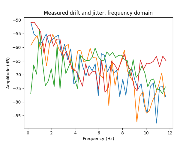
Drift and jitter are modeled as $f \cdot (1 + x)$ where $f$ is the static base frequency and $x$ is the deviation signal. The ratio $x / f$ is treated as an amplitude and converted to decibels, and this is what is meant by drift and jitter having a decibel value.

Cook also notes that drift and jitter also exhibit a small peak around the natural vibrato frequency, here around 3.5 Hz. Curiously, I don’t see any such peak in my data.

Synthesis can be done with interpolated value noise for drift and “clipped brown noise” for jitter, added together. Interpolated value noise is downsampled white noise with sine wave segment interpolation. Clipped brown noise is defined as a random walk that can’t exceed the range [-1, +1].

Vibrato is, not surprisingly, a sine wave LFO. However, a perfect sine wave sounds pretty unrealistic. Based on visual inspection of vibrato data, I multiplied the sine wave by random amplitude modulation with interpolated value noise. The frequency of the interpolated value noise is the same as the vibrato frequency.

A plot labeled "Measured vibrato, time domain." The X-axis is a time span of four seconds, and the Y-axis is frequency. The vibrato is quite smooth, with a peak-to-peak amplitude of about 10 Hz and a frequency of about 4 Hz, but the peaks and troughs vary.

A plot labeled "Synthetic vibrato, time domain." Again, the X-axis is a time span of four seconds, and the Y-axis is frequency. It looks similar to the measured plot but a bit smoother.

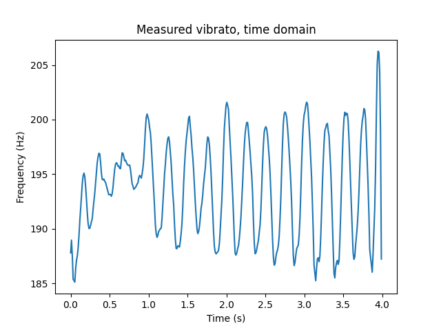
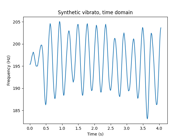
Also note that vibrato takes a moment to kick in, which is simple enough to emulate with a little envelope at the beginning of each note.

Portamento, overshoot, and preparation I couldn’t find much research on, so I sought to collect a good amount of data on them. I asked the singer to perform two-note melodies consisting of ascending and descending m2, m3, P4, P5, and P8, each four times, with instructions to use “natural portamento.” I then ran all the results through the pitch tracker and visually measured rough averages of preparation time, preparation amount, portamento time, overshoot time, and overshoot amount. Here’s the table of my results.

Interval	Prep. time	Prep. amount	Port. time	Over. time	Over. amount
m3 ascending	0.1	0.7	0.15	0.2	0.5
m3 descending	no preparation		0.1	0.3	1
P4 ascending	no preparation		0.1	0.3	0.5
P4 descending	no preparation		0.2	0.2	1
P5 ascending	0.1	0.5	0.2	no overshoot
P5 descending	no preparation		0.2	0.1	1
P8 ascending	0.1	1	0.25	no overshoot
P8 descending	no preparation		0.15	0.1	1.5

As one might expect, portamento time gently increases as the interval gets larger. There is no preparation for downward intervals, and spotty overshoot for upward intervals, both of which make some sense physiologically – you’re much more likely to involuntarily relax in pitch rather than tense up. Overshoot and preparation amounts have a slight upward trend with interval size. The overshoot time seems to have a downward trend, but overshoot measurement is pretty unreliable.

Worth noting is the actual shape of overshoot and preparation.

A plot titled "Portamento, ascending m3" showing four measured pitch signals. The X-axis is time and the Y-axis is frequency measured in MIDI note, which starts at about 52 and jumps to about 55. Preparation is only clearly visible for two of the signals, but it's about 70 cents.

A plot titled "Portamento, descending m3" showing four measured pitch signals. The X-axis is time and the Y-axis is frequency measured in MIDI note, which starts at about 55 and jumps to about 52. Overshoot is clearly visible for three of the four signals, nearly a semitone and a half.

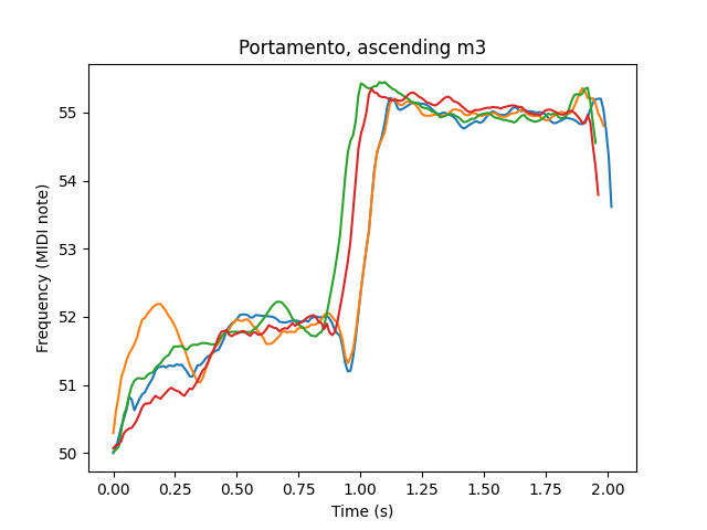
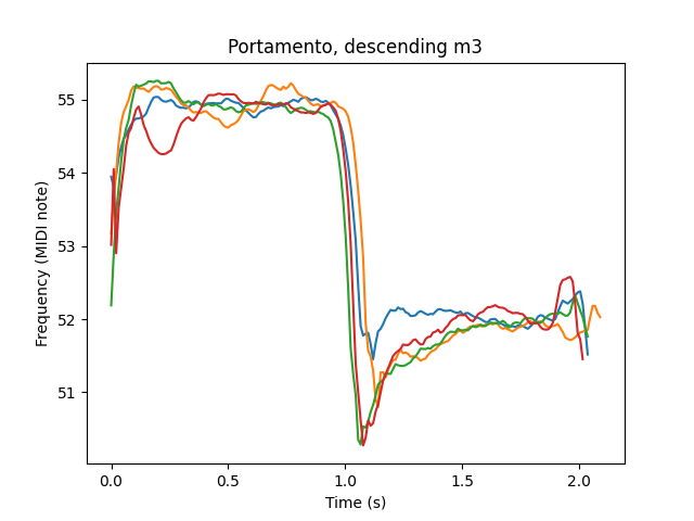
In OddVoices, I model these three pitch phenomena by using quarter-sine-wave segments, and assuming no overshoot when ascending and no preparation when descending.

Further updates

Pitch detection and pitch contours consumed most of my time and energy recently, but there are a few other updates too.

As mentioned earlier, I registered the domain oddvoices.org, which currently hosts a copy of the OddVoices Web interface. The Web interface itself looks a little bland – I’d even say unprofessional – so I have plans to overhaul it especially as new parameters are on the way.

The README has been heavily updated, taking inspiration from the article “Art of README”. I tried to keep it concise and prioritize information that a casual reader would want to know.

References

[Noll1966]

Noll, A. Michael. 1966. “Cepstrum Pitch Determination.

[Rabiner1977]

Rabiner, L. 1977. “On the Use of Autocorrelation Analysis for Pitch Detection.”

[Dziubinski2004] (1,2)

Diubinski, M. and Kostek, B. 2004. “High Accuracy and Octave Error Immune Pitch Detection Algorithms.”

[McLeod2008]

McLeod, Philip. 2008. “Fast, Accurate Pitch Detection Tools for Music Analysis.”

[Kumaraswamy2015]

Kumaraswamy, B. and Poonacha, P. G. 2015. “Improved Pitch Detection Using Fourier Approximation Method.”

[Cook1996]

Cook, P. R. 1996. “Identification of Control Parameters in an Articulatory Vocal Tract Model with Applications to the Synthesis of Singing.”

[Lai2009]

Lai, Wen-Hsing. 2009. “An F0 Contour Fitting Model for Singing Synthesis.”

[Lee2006]

Lee, Kyogu. 2006. “Automatic Chord Recognition from Audio Using Enhanced Pitch Class Profile.”

[McGonegal1977]

McGonegal, Carol A. et al. 1977. “A Subjective Evaluation of Pitch Detection Methods Using LPC Synthesized Speech.”

OddVoices Dev Log 2: Phase and Volume

Nathan Ho

2022-01-23

This is the second in an ongoing series of dev updates about OddVoices, a singing synthesizer I’ve been developing over the past year. Since we last checked in, I’ve released version 0.0.1. Here are some of the major changes.

New voice!

Exciting news: OddVoices now has a third voice. To recap, we’ve had Quake Chesnokov, a powerful and dark basso profondo, and Cicada Lumen, a bright and almost synth-like baritone. The newest voice joining us is Air Navier (nav-YEH), a soft, breathy alto. Air Navier makes a lovely contrast to the two more classical voices, and I’m imagining it will fit in great in a pop or indie rock track.

Goodbye GitHub

OddVoices makes copious use of Git LFS to store original recordings for voices, and this caused some problems for me this past week. GitHub’s free tier caps the amount of Git LFS storage and the monthly download bandwidth to 1 gigabyte. It is possible to pay $5 to add 50 GB to both storage and bandwidth limits. These purchases are “data packs” and are orthogonal to GitHub Pro.

What’s unfortunate is that all downloads by anyone (including those on forks) contribute to the monthly download bandwidth, and even worse, downloads from GitHub Actions do also. I am easily running CI dozens of times per week, and multiplied by the gigabyte or so of audio data, the plan is easily maxed out.

A free GitLab account has a much more workable storage limit of 10 GB, and claims unlimited bandwidth for now. GitLab it is. Consider this a word of warning for anyone making serious use of Git LFS together with GitHub, and especially GitHub Actions.

Goodbye MBR-PSOLA

OddVoices, taking after speech synthesizers of the 90’s, is based on concatenation of recorded segments. These segments are processed using PSOLA, which turns them into a sequence of frames (grains), each for one pitch period. PSOLA then allows manipulation of the segment in pitch, time, and formants, and sounds pretty clean. The synthesis component is also computationally efficient.

One challenge with a concatenative synthesizer is making the segments blend together nicely. We are using a crossfade, but a problem arises – if the phases of the overlapping frames don’t approximately match, then unnatural croaks and “doubling” artifacts happen.

There is a way to solve this: manually. If one lines up the locations of the frames so they are centered on the exact times when the vocal folds close (the so-called “glottal closure instant” or GCI), the phases will match. Since it’s difficult to find the GCI from a microphone signal, an electroglottograph (EGG) setup is typically used. I don’t have an EGG on hand, and I’m working remotely with singers, so this solution has to be ruled out.

A less daunting solution is to use FFT processing to make all phases zero, or set every frame to minimum phase. These solve the phase mismatch problem but sound overtly robotic and buzzy. (Forrest Mozer’s TSI S14001A speech synthesis IC, memorialized in chipspeech’s Otto Mozer, uses the zero phase method – see US4214125A.) MBR-PSOLA softens the blows of these methods by using a random set of phases that are fixed throughout the voice database. Dutoit recommends only randomizing the lower end of the spectrum while leaving the highs untouched. It sounds pretty good, but there is still an unnatural hollow and phasey quality to it.

I decided to search around the literature and see if there’s any way OddVoices can improve on MBR-PSOLA. I found [Stylianou2001], which seems to fit the bill. It recommends computing the “center” of a grain, then offsetting the frame so it is centered on that point. The center is not the exact same as the GCI, but it acts as a useful stand-in. When all grains are aligned on their centers, their phases should be roughly matched too – and all this happens without modifying the timbre of the voice, since all we’re doing is a time offset.

I tried this on the Cicada voice, and it worked! I didn’t conduct any formal listening experiment, but it definitely sounded clearer and lacking the weird hollowness of the MBROLA voice. Then I tried it on the Quake voice, and it sounded extremely creaky and hoarse. This is the result of instabilities in the algorithm, producing random timing offsets for each grain.

Frame adjustment

Let $x[t]$ be a sampled quasiperiodic voice signal with period $T$, with a sample rate of $f_s$. We round $T$ to an integer, which works well enough for our application. Let $w[t]$ be a window function (I use a Hann window) of length $2T$. Brackets are zero-indexed, because we are sensible people here.

The PSOLA algorithm divides $x$ into a number of frames of length $2T$, where the $n$-th frame is given by $s_n[t] = w[t] x[t + nT]$.

Stylianou proposes the “differentiated phase spectrum” center, or DPS center, which is computed like so:

\begin{equation*} \eta = \frac{T}{2\pi} \arg \sum_{i = -T}^{T - 1} s_n^2[t] e^{2 \pi j t / T} \end{equation*}

$\eta$ is here expressed in samples. The DPS center is not the GCI. It’s… something else, and it’s admitted in the paper that it isn’t well defined. However, it is claimed that it will be close enough to the GCI, hopefully by a near-constant offset. To normalize a frame on its DPS center, we recalculate the frame with an offset of $\eta$: $s'_n[t] = w[t] x[t + nT + \text{round}(\eta)]$.

The paper also discusses the center of gravity of a signal as a center close to the GCI. However, the center of gravity is less robust than the DPS center, as it can be shown that the center can be computed from just a single bin in the discrete Fourier transform, whereas the DPS center involves the entire spectrum.

Here’s where we go beyond the paper. As discussed above, for certain signals $\eta$ can be noisy, and using this algorithm as-is can result in audible jitter in the result. The goal, then, is to find a way to remove noise from $\eta$.

After many hours of experimenting with different solutions, I ended up doing a lowpass filter on $\eta$ to remove high-frequency noise. A caveat is that $\eta$ is a circular value that wraps around with period $T$, and performing a standard lowpass filter will smooth out discontinuities produced by wrapping, which is not what we want. The trick is to use an encoding common in circular statistics, and especially in machine learning: convert it to sine and cosine, perform filtering on both signals, and convert it back with atan2. A rectangular FIR filter worked perfectly well for my application.

Overall the result sounds pretty good. There are still some minor issues with it, but I hope to iron those out in future versions.

Volume normalization

I encountered two separate but related issues regarding the volume of the voices. The first is that the voices are inconsistent in volume – Cicada was much louder than the other two. The second, and the more serious of the two, is that segments can have different volumes when they are joined, and this results in a “choppy” sound with discontinuities.

I fixed global volume inconsistency by taking the RMS amplitude of the entire segment database and normalizing it to -20 dBFS. For voices with higher dynamic range, this caused some of the louder consonants to clip, so I added a safety limiter that ensures the peak amplitude of each frame is no greater than -6 dBFS.

Segment-level volume inconsistency can be addressed by examining diphones that join together and adjusting their amplitudes accordingly. Take the phoneme /k/, and gather a list of all diphones of the form k* and *k. Now inspect the amplitudes at the beginning of k* diphones, and the amplitudes at the end of *k diphones. Take the RMS of all these amplitudes together to form the “phoneme amplitude.” Repeat for all other phonemes. Then, for each diphone, apply a linear amplitude envelope so that the beginning frames match the first phoneme’s amplitude and the ending frames match the second phoneme’s amplitude. The result is that all joined diphones will have a matched amplitude.

Conclusion

The volume normalization problem in particular taught me that developing a practical speech or singing synthesizer requires a lot more work than papers and textbooks might make you think. Rather, the descriptions in the literature are only baselines for a real system.

More is on the way for OddVoices. I haven’t yet planned out the 0.0.2 release, but my hope is to work on refining the existing voices for intelligibility and naturalness instead of adding new ones.

References

[Stylianou2001]

Stylianou, Yannis. 2001. “Removing Linear Phase Mismatches in Concatenative Speech Synthesis.”