Mother wavelet

…which is a square-integrable function \(\psi \in L^2(\mathbb{R})\). The mother wavelet may be real-valued \(\psi: \mathbb{R} \rightarrow \mathbb{R}\) or generally complex-valued \(\psi: \mathbb{R} \rightarrow \mathbb{C}\). Mother wavelets are often, but not always, subject to the following rules:

1. It must have a norm of 1: \(||\psi|| = 1\).

2. It must have an integral of 0, i.e. no dc bias:

We’ll break both these rules, but I introduce them to assist with building intuition. These connect to the bandpass filter, because a reasonable definition of a bandpass filter is that 1. its dc bias is zero and 2. its magnitude response tapers off to zero for infinite frequencies. The first requirement is the above integral rule, and the second requirement is automatically satisfied for us, because functions in \(L^2(\mathbb{R})\) always have tapered magnitude spectra. Thus square-integrable functions not only have time locality, but also frequency locality.

A common way to produce a wavelet is to start with a sinusoid and envelope it with a tapered function, such as \(\psi(t) = e^{-t^2} \sin(3 t)\). I’ve left out the normalization factor in the formula that would ensure \(||\psi|| = 1\), but other than that this fits all the criteria.

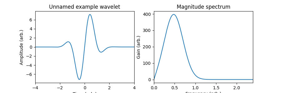
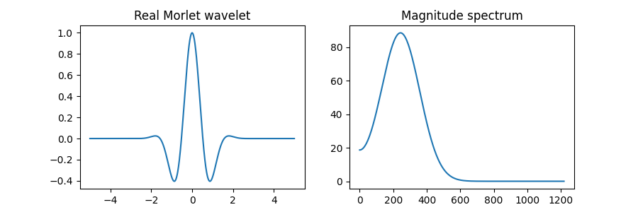
The wavelet actually doesn’t need to be a bandpass, but rather somewhat bandpass-shaped. If it has a peak at a nonzero frequency and dips at least a little as you approach dc, it’s a useful wavelet. The wavelet \(\psi(t) = e^{-t^2} \cos(3 t)\) is the real Morlet wavelet. As you can see from the value of its magnitude spectrum at 0 frequency, its dc bias is not exactly zero, but still looks reasonably like a bandpass. This is a very common wavelet, and the one we’ll be using for many examples.

Wavelets can also be complex-valued, such as in the complex Morlet wavelet: \(\psi(t) = \exp(3jt - t^2)\).

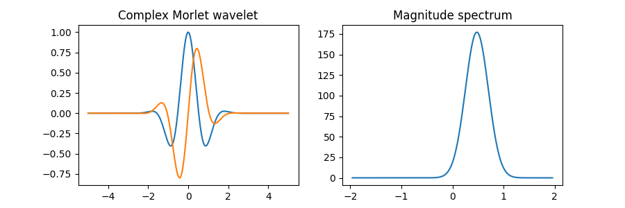
[TODO: Vertical and horizontal scales may be wrong on the frequency-domain plots.]

As far as I can tell real wavelets are slightly more common than complex wavelets, although both are used. We’ll stick to the real Morlet wavelet and talk about other established wavelets in a later section.

Time-shifting the mother wavelet

Given a square-integrable input signal \(f\), consider the inner product of \(f\) with \(\psi\):

To gain some intuition over what this inner product is doing, it “analyzes” \(f\) with \(\psi\) and produces a single complex number that gives us information about the similarity of \(f\) and \(\psi\). If \(f\) has a lot of energy exactly where \(\psi\) has energy, then \(\langle f, \psi \rangle\) is likely to be higher in magnitude. If \(f\) and \(\psi\) don’t really line up much then the inner product will be close to zero.

However, because of \(\psi\)’s time-locality, this analysis only gives us information about a certain window of time. To gain more information about \(f\), let’s shift the mother wavelet around in time \(t \in \mathbb{R}\):

We can then take the inner product \(\langle f, \psi_t \rangle\) to analyze \(f\) at any time. If we expand the inner product

then sharp readers will notice that, as a function of \(t\), \(\langle f, \psi_t \rangle\) is just convolution of \(f\) with the complex conjugate of the mother wavelet \(\psi\). Since we are convolving \(f\) with a wavelet, this is just a bandpass filter — nothing exciting yet.

Scaling the mother wavelet

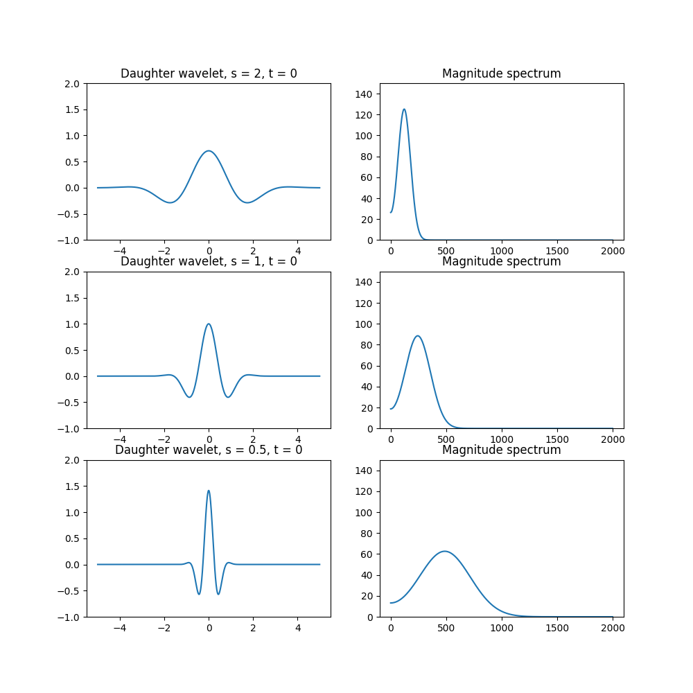
The mother wavelet is also frequency-local, so evaluating \(\langle f, \psi_t \rangle\) for every \(t\) only really gives us information about \(f\) in one frequency band. Here is where the wavelet magic comes in. We scale the mother wavelet in time to change its frequency range:

where \(s \neq 0\) is the scaling factor and \(t\) is the time shift applied after scaling. \(s > 1\) expands or dilates the wavelet, \(0 < s < 1\) compresses it, \(s < 0\) performs time-reversal and scaling. In practice, negative scales \(s < 0\) are often ignored. The full gamut of functions \(\psi_{s,t}\) gives us the full set of daughter wavelets.

The scale multiplies the center frequency of the bandpass-shaped filter by a factor \(1/s\). So when you hear high scale, think lower frequency, and vice versa.

It is generally desirable to have all daughter wavelets retain unit norm. From the properties of the norm, we multiply the daughter wavelet by the following corrective factor.

(Note that sometimes this factor is written as \(1/|s|\) or omitted entirely, depending on the application.)

A property of the Fourier transform states that time-scaling a function around 0 also scales its Fourier transform. When a wavelet is scaled by \(s\), its frequency response is scaled by \(1 / s\). (Its amplitude also changes.) Thought of as a filter, scaling moves around its center frequency.

Its bandwidth is also scaled by the same amount, so its Q remains constant. For this reason the CWT overlaps with some versions of the Constant-Q Transform, but alas CQT means different things depending on who you talk to.

In audio, it’s common to view filter frequency responses on a log-log scale, like in typical parametric equalizers. Here are a few frequency responses of selected Morlet wavelets with logarithmic frequency and decibel units:

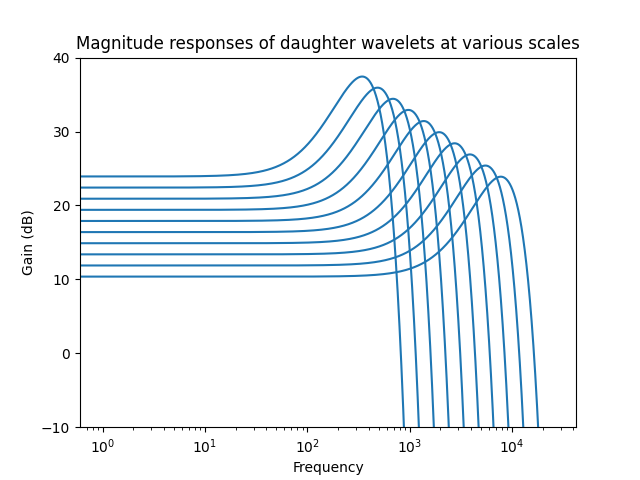
As you can see, they are all formed by a rigid “diagonal” translation of the mother wavelet. The horizontal component of this translation is the result of frequency scaling, while the vertical component is just a change in gain.

Definition of the CWT

We now have all the information we need to define the CWT. With the inner product and the daughter wavelets defined, the formula for expressing the transform is particularly terse.

While the Fourier transform turns a one-dimensional function of time into a one-dimensional function of frequency, the CWT produces a two-dimensional function, with the parameters of scale and time shift. There is no discretization here: \(\tilde{f}(s, t)\) is defined for every \(s \neq 0\) and every real \(t\).

Being complex, \(\tilde{f}(s, t)\) has both phase and magnitude. (If the signal and wavelet are real-valued, \(\tilde{f}(s, t)\) is of course real, but it can be negative.) If we plot the magnitude \(|\tilde{f}(s, t)|\) as a two-dimensional image with time on the horizontal axis and scale on the vertical axis, we produce something called the scalogram. The visual of the scalogram is extremely useful for understanding the CWT and its variants.

If we take this rectangular-windowed sine wave sweep:

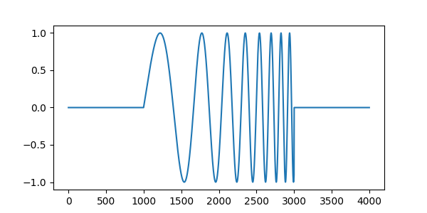
and the real Morlet wavelet, we may view our first scalogram:

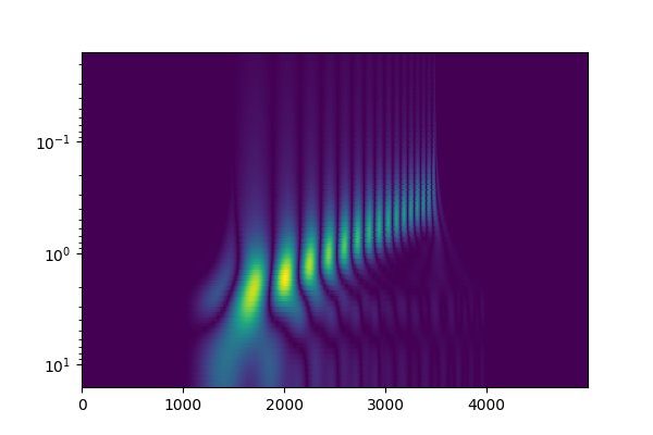
[TODO: There might be windowing artifacts in this since I had to truncate the wavelet for practical computation.]

I’ve followed two common conventions in scalograms: a log scale for the vertical axis, and to place smaller scales (and therefore higher frequencies) towards the top.

You can see a diagonal line here that looks pretty close to straight, indicating that the frequency of the sine wave sweep I put in is exponential. We could have also learned that from a spectrogram. However, a typical spectrogram would show a continuous line; here the scalogram breaks up the sweep into a discrete set of “hot spots.” This scalogram’s time resolution divides the sine wave into individual pulses, while still being aware of its changing frequency. However, the time-frequency resolution situation is dependent on the choice of wavelet.

Keep in mind that scalograms, like spectrograms, typically depict only magnitude and not phase, so they don’t contain all the information that the CWT provides.

Inverse Continuous Wavelet Transform

With the CWT established, musicians familiar with FFT processing via the phase vocoder are likely itching to start modifying and inverting the CWT to create scalogram-based effects. Not so fast, soldier.

My own introduction to time-frequency transforms was through FFT in computer music, and I imagine that’s likely the case for much of my audience. It was a rude awakening for me to learn that the Fourier transform is rather special, and in general not all time-frequency transforms are actually invertible in theory and practice. Many wavelet transform variants fail to be invertible at all.

The CWT, the primordial organism that every wavelet-like transform descends from, is in fact invertible. Sort of, kind of, sometimes. If I give you the CWT \(\tilde{f}\) of a signal, the Inverse Continuous Wavelet Transform (ICWT) allows us to recover \(f\). However, there are some important caveats:

• It is easy to come up with \(\tilde{f}\) that do not have any inverse CWT. If I modify \(\tilde{f}\) even a tiny amount, there may not be any \(f\) that corresponds to it, because the CWT is highly redundant. This is in stark contrast to, say, the discrete Fourier transform, where any modification done in the Fourier domain will always have a valid inverse.

• Actually computing the ICWT is difficult in the general case. Some wavelets make it easier. [TODO: explain which ones]

• A constant bugbear in the design of FFT pitch shifters, etc. is the problem of phase coherence. In the case of the CWT, phases are even more unintuitive and difficult to work with than they are in FFT.

• If \(\psi\) has a dc offset of 0, then the CWT can’t possibly capture any information about the dc offset of \(f\), and the ICWT cannot recover it. This isn’t a huge problem for audio signals where dc offsets are generally considered a nuisance, but it’s worth noting to avoid confusion.

Overall, my impression from the literature is that the ICWT is not very common. The CWT is used most frequently for analysis and visualization, and not so much for processing.

Due to all the thorny problems involved, I won’t cover the ICWT in depth. However, we will later discuss an easily invertible variant of the CWT called Multiresolution Analysis.

Quantizing frequency

Generally there’s not much use in really fine-grained shifts of \(t\) that are less than a sample, so it’s okay to assume that \(t\) is an integer.

In the case of \(s\), a common approach is to use exponentially spaced scaling factors, such as \(s = 2^{k / d}\) where \(k\) is an integer index and \(d\) is a number of divisions we care about per octave. For analysis of Western music, setting \(d\) to a multiple of 12, such as 24 or 48, is a possible choice.

There is a natural lower limit to \(s\), because at some point the daughter wavelets are so squashed that they have very little energy below Nyquist. As mentioned above, this bound is \(s > F / \text{Nyquist}\) where the mother wavelet has little to no energy above \(F\). There is nothing stopping you from using smaller \(s\) values, but the discretized daughter wavelets will just be aliased garbage and won’t tell you anything that higher \(s\) values don’t do.

In theory, \(s\) has no upper limit. As it approaches infinity the daughter wavelets analyze lower and lower frequencies and approach dc. However, in all practical applications you have a lower bound on useful frequencies. In audio, this is usually the 20 Hz lower limit on human hearing.

Although it is common in applications to use exponentially spaced \(s\) values, be aware that it isn’t a requirement. If you want, you can use linear frequencies, or mel frequencies, or Bark frequencies, or a small set of hand-picked frequencies (such as DTMF tones).

SciPy’s scipy.signal.cwt implements the DT-CWT where \(t\) is set to all integer sample values, and the values of \(s\) are specified as an arbitrary array. (See docs.) Notably, SciPy does not provide an icwt that takes us back to the time domain.

Downsampling DT-CWT bands

To recap, we started by conceptualizing the CWT as an infinitely dense bank of bandpass filters on a continuous-time signal. With the DT-CWT we discretized the input signal, then we quantized the frequency bands, producing a finite bank of bandpass filters. At this point we have an algorithm with a straightforward computer implementation.

If you think about what happens for lower frequencies and larger values of \(s\), the signal formed by convolving with the corresponding daughter wavelets has little high-frequency energy. If the mother wavelet has little to no energy above a frequency \(F\), then the signal produced by bandpass-filtering the input at scale \(s\) is effectively bandlimited at \(F / s\). If \(F / s < \text{Nyquist} / 2\) then we don’t lose much information by downsampling the signal by a factor of two. So, for \(s \geq 2 F / \text{Nyquist}\) we only care about every other sample. As the signal is already quasi-bandlimited, the downsampling can be done by naively dropping every other sample; no additional filtering is required. Put another way, for suitably large \(s\) our set of daughter wavelets can be reduced by only considering \(\psi_{s,t}\) for even \(t\).

In general, for scale \(s\), the corresponding bandpassed signal can be downsampled by up to a factor of \(k\), where \(k = \left\lfloor \frac{sF}{\text{Nyquist}} \right\rfloor\). Since we compute the CWT through a stack of convolutions, we can reduce computational cost by just not computing the dropped samples in the first place.

Let’s consider a DT-CWT with 12 bands per octave where each \(s\) value has been downsampled by the maximum allowable integer factor. If we place a dot at every value of \(s\) and \(t\) corresponding to a daughter wavelet \(\psi_{s,t}\), we’ll get something lilke this:

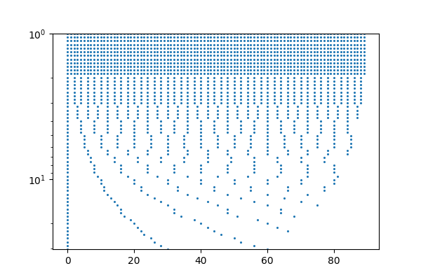
Thus, the result of the DT-CWT is a single complex value at each of these dots. While somewhat pretty-looking (reminiscent of driving by orchards in NorCal), this downsampling scheme is not done in practice because the data structure needed to store these points is tough to work with. The pattern of dots is ultimately periodic along the time axis, but the period is very long.

I wrote that the downsampling can be done up to a factor of \(k\), but it need not be exactly \(k\). A common approach is to round the downsampling factors down to integer powers of 2.

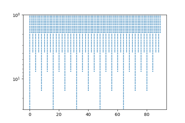
In exchange for slightly suboptimal downsampling, we have something much easier to work with. The pattern of dots has a short period, which is simply the time distance between samples in the bottom octave. (We still get all these benefits even if the spacing of \(s\) is not exponential.)

This variable-rate downsampling is more than just a shortcut to save space and kiloflops. It’s a fundamental component of our next topic:

Analysis with MRA

I’m going to assume real wavelets here. Modifications are necessary for complex wavelets, albeit only minor ones.

To implement MRA, we are given a reconstruction lowpass filter with impulse response \(h[t]\) where \(t \in \mathbb{Z}\) Practical implementations require \(h\) to be FIR; IIR lowpass filters are also of use since they can be truncated.

We can’t just pick any \(h\); it has to satisfy certain special properties which will be shortly described. One is that the cutoff of \(h\) should be half Nyquist, or one quarter of the sample rate. [TODO: note amplitude normalization.] There is no requirement that \(h[t]\) is causal, meaning it may be nonzero for \(t < 0\). In e.g. image processing there is no notion of “causality,” but in real-time audio this adds a complication, one that we’ll talk about later.

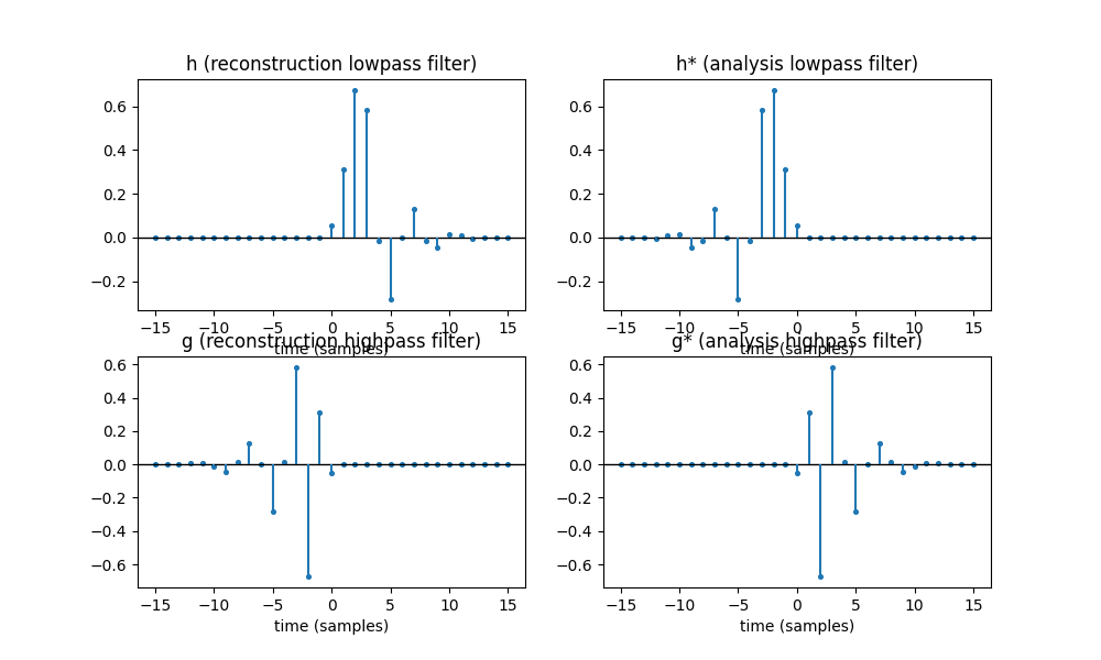
From the reconstruction lowpass filter we produce three other filters:

Here’s what they look like:

[TOOD: fix crashing text]

\(h^*\) is the time-reversal of the filter about \(t = 0\). Filter nerds can verify that the convolution \(h * h^*\) produces a zero phase lowpass filter whose magnitude spectrum is the square of the magnitude spectrum of \(h\); this is the exact same principle as that of forward-backward filtering. (The superscript \(^*\) is not quite the complex conjugate but rather the adjoint of the filter, which I don’t have the space to describe. Don’t confuse it with the centered \(*\), which is plain old convolution.)

\(g\) time-reverses \(h\) and flips the sign of every other coefficient, and \(g^*\) in turn time-reverses \(g\). These are highpass filters: multiplying (modulating) a signal with a sine wave at Nyquist produces a spectral inversion. Again \(g * g^*\) is zero phase, and its magnitude spectrum is the square of \(g\)’s magnitude spectrum.

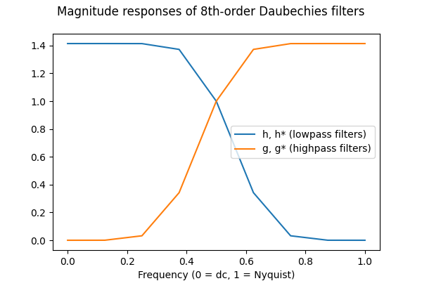
The filters I’ve plotted above in this example are rather special ones, with \(h\) being derived from the 8th-order Daubechies wavelet. These are FIR filters and they vanish to zero outside of the range I’ve plotted. Also, noting the ranges on the X-axes, we have \(h[t] = 0\) for \(t < 0\), so \(h\) and \(g^*\) are causal; this is not necessarily true of all filters. We can plot their magnitude responses on a linear-linear scale to confirm that these are indeed low and highpass filters whose cutoffs are half Nyquist:

[TODO: add zero padding prior to FFT for smoother response]

\(g\) and \(g^*\) have the same magnitude responses and so do \(h\) and \(h^*\); between each adjoint pair the phase responses (not shown) are sign flips of each other.

We define the linear (but not time-invariant!) operators \(S_\Downarrow\) and \(S_\Uparrow\). \(S_\Downarrow\) downsamples a signal by 2x by discarding every other sample: \((S_\Downarrow f)[t] = f[2t]\). \(S_\Uparrow\) upsamples a signal 2x by inserting zeros: \((S_\Uparrow f)[2t] = f[t]\) and \((S_\Uparrow f)[2t + 1] = 0\). In the frequency domain, \(S_\Downarrow\) folds the top half of the digital signal down to the top half, and \(S_\Uparrow\) mirrors the entire spectrum around half Nyquist.

We are now ready to define the Fast Wavelet Transform:

I know you’re looking for a block diagram, so here it is, topping out at \(J = 3\):

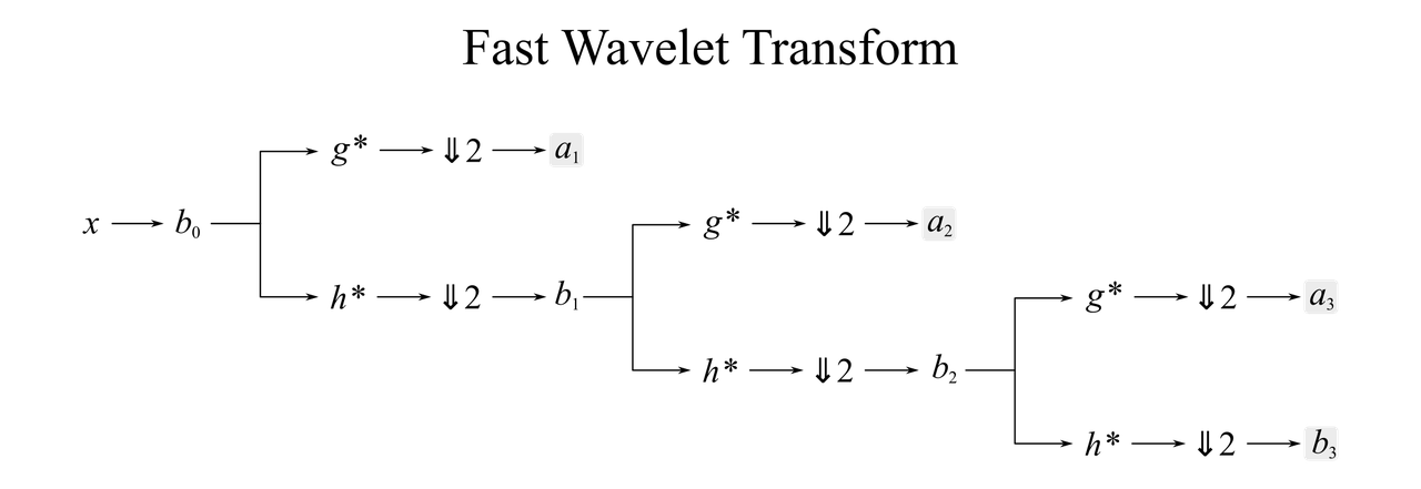
The output signals are outlined with gray boxes. Note that the \(a_\cdot\) and \(b_\cdot\) steps are just variable names, not actual filters or processing steps.

The downsampling operator naturally introduces aliasing, but since \(h^*\) is a lowpass, it acts as an antialiasing filter by attenuating the high frequencies. Complementarily, \(g^*\) filters out the low frequencies, and the downsampling operator mirrors these high frequencies around half Nyquist.

If we only want to use MRA to analyze the signal, then we can just take our downsampled signals and be done with it. But a magical property of the MRA states that, under certain conditions, it is possible to use these analysis signals to recover \(u^0\).

Block diagram block diagram block diagram:

In plain English, we take the lowpass/highpass pair, upsample them, and convolve them with the reconstruction lowpass and highpass filters. Then we add them together to try to reconstruct the highpass signal.

I wrote that we try to reconstruct \(b_0\). In reality, \(h[t]\) must be designed in the first place so that perfect reconstruction is possible. In practice, someone implementing an MRA will know a priori that \(h[t]\) is suited for this purpose. The takeaway is that you can’t plug random lowpass filters into MRA and get perfect reconstruction.

Implementation details

This algorithm is almost implementable right out of the block diagram, but we first need to discuss a minor optimization and a major caveat.

[TODO: polyphase filtering, latency compensation in non-causal filters]

Connecting MRA to the CWT, part 1: the intuition

It is entirely understandable if you are having trouble understanding the relationship to wavelets here. That was the case for me when I first looked at the FWT algorithm. However, as promised, there is a deep connection between these two transforms. The MRA-CWT linkage gets a little technical, and we’ll see a more precise treatment in the next section, but I want to set it up with a visual explanation first.

The recursive downsampling scheme results in multiple streams at different sampling rates, all of which are power-of-two divisions of the original signal’s sample rate. If we place a dot at the time of every sample, and write the different streams as rows, we get a familiar diagram:

[TODO: MRA dots diagram]

If you guessed that the MRA values are in fact inner products produced by the DT-CWT at power-of-two scales, you win a point:

This is quite beautiful, but why this is the case isn’t obvious. To gain some intuition, we’ll examine what the MRA is doing in a filter theory sense. As a jumping-off point, we’ll start with the signal \(a_2\) produced by the FWT. \(a_2\) is the result of the following operations on the input signal:

1. Lowpass filter with cutoff \(f_N/2\) and downsample by a factor of 2.

2. Highpass filter with cutoff \(f_N/4\) and downsample again by a factor of 2. (Here \(f_N\) is the Nyquist frequency of the original signal prior to downsampling. Relative to the current signal’s sample rate, the cutoffs of these filters are always half Nyquist; a common cuss word for these is “half-band filter.”)

If we ignore the downsampling operations for a moment, we find that this is a highpass filter followed by a lowpass filter, which is a bandpass that roughly isolates the frequency content in the range \([f_N / 4, f_s / 2]\). What about \(a_3\)?

1. Lowpass filter with cutoff \(f_N/2\) and downsample by a factor of 2.

2. Lowpass filter with cutoff \(f_N/4\) and downsample by a factor of 2.

3. Highpass filter with cutoff \(f_N/8\) and downsample by a factor of 2.

Again, if the downsampling operations are ignored, this is a bandpass filter that isolates the range \([f_N / 8, f_s / 4]\). In general, we may conclude that in the absence of downsampling, the \(a_m\) signals for \(m > 1\) are the result of a bandpass filter with a rough passband of \([2^{-m - 1} f_s, 2^{-m} f_s]\).

The connection to the CWT should start to feel closer now that bandpass filters have shown up, but we aren’t quite home free yet; we still have those pesky downsampling operations, which being non-time-invariant are not guaranteed to commute with other operations. It turns out that they do commute approximately, and we can conceptually move all the downsampling to the end: [3]

1. Bandpass filter to the range \([2^{-m - 1} f_N, 2^{-m} f_N]\).

2. Downsample by a factor of \(2^{-m}\). As the signal only has significant energy up to \(2^{-m} f_N\), there’s no aliasing.

3. Downsample by a factor of 2. This folds the upper half of the spectrum and spectrally inverts it to the range \([0, 2^{-m - 1} f_N]\).

So the MRA really does have bandpass filter-like functionality, and in step 2 it downsamples out redundant information as we discussed in the DT-CWT. Step 3 isn’t something we’ve seen before — it further compresses the DCWT band with an additional downsampling stage. As this just amounts to leaving out half the dots on the DCWT, we are still technically evaluating the DCWT, just at fewer locations. The fact that we are able to omit half the points without information loss is specific to the shape of the bandpass filter; if its lower band edge was any lower than \(2^{-m - 1} f_N\) then the signal crashes into itself. (This may be the case if the wavelet is not orthogonal, such as the Morlet wavelet.)

The impulse response of the bandpass filter is of course a daughter wavelet. With the information we have, we can compute the daughter wavelet itself: it is a cascade of \(m\) analysis lowpass filters at increasing power-of-two scales, followed by one last highpass filter at scale \(m\). Since all daughter wavelets are related by scaling and time-shifting, we can compute the mother wavelet to arbitrary time precision by increasing \(m\) as high as we want.

I didn’t mention the final \(b_J\) signal at the bottom of the FWT. All you need to know for intuition is that this signal’s chain is just lowpasses, and therefore it isn’t actually part of the DT-CWT. To properly describe it we need yet another new concept (sorry), that of the scaling function — and we’ll leave that for the nerds to peruse in the next section.

Connecting MRA to the CWT, part 2: the math

This section is optional. [TODO: This section also probably has some mistakes.]

Welcome, nerds. A scaling function is denoted \(\phi(t)\), a square-integrable function \(\mathbb{R} \rightarrow \mathbb{C}\). Like a mother wavelet, it has both time- and frequency-locality. Unlike a wavelet, \(\phi(t)\) has a dc value (integral) of 1 instead of 0, so the frequency locality is around dc. The scaling function is a lowpass rather than a bandpass; there is no specific requirement of what its cutoff is.

For convenience, we define a dilation operator \(D\), which stretches out a function by factor of 2 and retains its norm:

and a time-shift operator, which displaces the function in time by an integer shift:

Scaling functions do not exist for general wavelets as far as I understand; they are only used in conjunction with orthogonal wavelets in the context of MRA. (Many wavelet resources fail to make this clear, and it tripped me up a lot.) An orthogonal wavelet has exactly one associated scaling function, and a scaling function has exactly one asssociated orthogonal wavelet if it satisfies a property called the two-scale relation:

where \(h[t]\) is an integer-indexed sequence of real numbers. In English, the dilation of \(\phi\) is a linear combination of copies of the original \(\phi\) translated by integer time shifts. The coefficients \(h[t]\) are precisely the reconstruction lowpass filter used in the FWT. Note that \(h * \phi_{2,0}\) is a mild abuse of notation because \(h\) is a discrete signal and \(\phi_{}\) is a continuous signal; to make this formally valid imagine that \(h\) is realized as train of Dirac delta functions at integer time values (and therefore its Fourier transform is periodic).

Some wavelet schemes start with \(h[t]\) and use that to define the scaling function. Others go in the opposite direction, starting with \(\phi(t)\) and deriving \(h[t]\):

In either case, the final piece of the puzzle, which you have likely been anticipating if you made it this far, is to connect \(\phi(t)\) to the actual mother wavelet \(\psi(t)\) ([Mallat1999], Theorem 7.3):

[TODO: Above formula may be sligthly incorrect, check normalization factor.]

Thus the mother wavelet is the combination of the lowpass filter \(\phi\) and the highpass filter \(g\), squashed by a factor of two. That a lowpass and highpass compose to form a bandpass should square with our intuition about wavelets.

With these three equations, we can convert among MRA filter coefficients, wavelets, and scaling functions. Converting between the three is not guaranteed to be simple — sometimes \(h\) can be derived but \(\phi\) and \(\psi\) lack a closed form, and other times we’re given \(\psi\) or \(\phi\) and we need numerical methods to find \(h\). In all cases, remember that these conversions only make sense if the following equivalent statements are true: the wavelet is orthogonal, the scaling function satisfies the two-scale relation, and the filter admits perfect reconstruction.

Complicated? Sure. Fortunately, these aren’t tools you’ll need much for typical use and implementation of FWT. In many cases, you’re just given \(h\). I’ve done this excursion into the math because I wanted an explanation that personally makes sense to me.

Morlet wavelet (Gabor wavelet)

[Morlet wavelet diagram]

Real or complex, infinite support, not orthogonal.

The Morlet wavelet is likely the most commonly used wavelet for the CWT. It has both real and complex versions. The real version is formed by enveloping a cosine wave with a Gaussian:

where \(\omega\) determines the Q factor of the filter, with higher \(\omega\) resulting in higher Q. The complex version replaces the cosine wave with a complex sinusoid:

Haar wavelet

[Haar wavelet & scaling function diagram]

Real, finite support, orthogonal.

The Haar wavelet predates the wavelet transform by decades, when it formed the basis of the Haar transform. It is a rectangular-shaped “wiggle:”

Its scaling function is even simpler, a rectangular bump:

It can be confirmed visually that \(\phi(2t) = (\phi(t) + \phi(t - 1)) / 2\), so the filter coefficients are \(h = \frac{1}{\sqrt{2}}[1,\,1]\).

Shannon wavelet

[Shannon wavelet & scaling function diagram]

Real, infinite support, orthogonal.

The Shannon wavelet is the wavelet answer to the ideal filter, or sinc filter. It’s only really useful as a theoretical ideal, not as a practical wavelet. It is easiest to define with its scaling function:

Daubechies wavelets

[Daubechies wavelets & scaling functions diagram]

Real, finite support, orthogonal.

The Daubechies wavelets are common choices for MRA. The \(n\) th-order Daubechies wavelet’s filter has length \(2n\); the case \(n = 1\) is the Haar wavelet.

The Daubechies wavelets are most easily specified as filter coefficients, but even they requires a fairly intricate numerical algorithm. Fortunately, you likely don’t need to implement that – SciPy has scipy.signal.daub, which gives you the FIR filter coefficients. \(\phi(t)\) and \(\psi(t)\) have no closed form, and generally have a complex fractal structure. They look pretty trippy, especially for naturally occuring mathematical functions.

Mexican hat wavelet (Ricker wavelet)

[Mexican hat wavelet diagram]

Real or complex, infinite support, not orthogonal.

The Mexican hat wavelet (more boringly, the Ricker wavelet) is real:

Others

Other orthogonal wavelets include the Meyer wavelet, symlets, and coiflets. If you aren’t constrained by orthogonality, then practically any function with reasonable time and frequency locality can be used as a wavelet. For example, for audio some have used the gammatone or gammachirp functions as wavelets.