Audio Texture Resynthesis
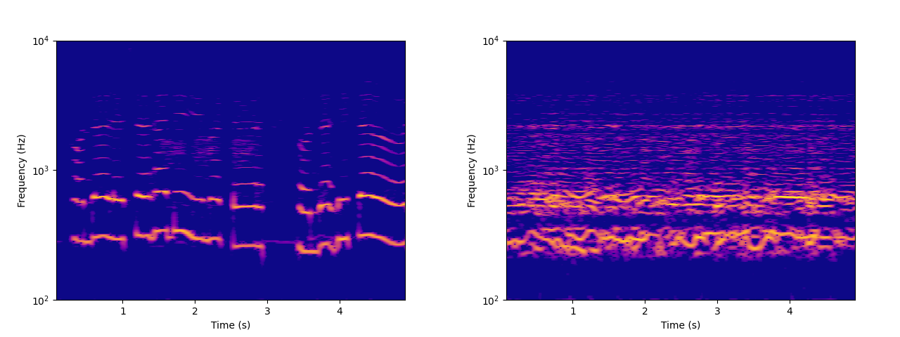
Left: spectrogram of a child singing. Right: spectrogram of resynthesized audio.
Background
I was alerted to audio texture resynthesis methods by a student of mine who was interested in the collaborative work of researcher Vincent Lostanlen, musician Florian Hecker, and several others [Lostanlen2019] [Lostanlen2021] [Andén2019] [Muradeli2022]. Their efforts are built on an analysis method called “Joint Time-Frequency Scattering” (JTFS) based on the Continuous Wavelet Transform. In an attempt to understand the work better, I binged a wavelet transform textbook, [1] implemented a simplified version of JTFS-based resynthesis, and and briefly exchanged emails with Lostanlen. His helpful answers gave me the impression is that while JTFS is a powerful analysis technique, resynthesis was more of a side project and there are ways to accomplish similar effects that are more efficient and easier to code without compromising too much on musicality.
Audio texture resynthesis has some history in computer music literature [Schwartz2010], and some researchers have used resynthesis to help understand how the human brain processes audio [McDermott2011].
After some experimentation with these methods, I found that it’s not too hard to build a simple audio texture resynthesizer that exhibits clear musical potential. In this blog post, I’ll walk through a basic technique for making such a system yourself. There won’t be any novel research here, just a demonstration of a minimum viable resynthesizer and my ideas on how to expand on it.
Algorithm
The above-mentioned papers have used fancy techniques including the wavelet transform and auditory filter banks modeled after the human ear. However, I was able to get decent results with a standard STFT spectrogram, then using phase reconstruction to get time-domain audio samples. The full process looks like this:
Compute a magnitude spectrogram \(S\) of the time-domain input signal \(x\). A fairly high overlap is advised.
Compute any number of feature vectors \(F_1(S),\, F_2(S),\, \ldots,\, F_n(S)\) and define their concatenation as \(F(S)\).
Initialize a randomized magnitude spectrogram \(\hat{S}\).
Use gradient descent on \(\hat{S}\) to minimize the error \(E(\hat{S}) = ||F(S) - F(\hat{S})||\) (using any norm such as the squared error).
Use phase reconstruction such as the Griffin-Lim algorithm on \(\hat{S}\) to produce a resynthesized signal \(\hat{x}\).
The cornerstone of making this algorithm work well is that we choose an \(F(S)\) that’s differentiable (or reasonably close). This means that the gradient \(\nabla E\) can be computed with automatic differentiation (classical backpropagation). As such, this algorithm is best implemented in a differentiable computing environment like PyTorch or Tensorflow.
The features \(F(S)\), as well as their relative weights, greatly affect the sound. If \(F(S)\) is highly time-dependent then the resynthesized signal will mimic the original in evolution. On the other hand, if \(F(S)\) does a lot of pooling across the time axis then the resynthesized signal will mostly ignore the large-scale structure of the input signal. I’m mostly interested in the latter case, where \(F(S)\) significantly “remixes” the input signal and disregards the overall structure of the original.
We will represent \(S\) as a 2D tensor where the first dimension is frequency and the second is time. As a matrix, each row is an FFT bin, and each column a frame.
If using a fancy alternative to the magnitude spectrogram such CWT or cochlear filter banks, you may have to do gradient descent all the way back to the time-domain samples \(x\). These analysis methods break down to linear frequency transforms that produce complex numbers followed by computing the absolute value of each bin, so differentiability is maintained.
Bin-specific statistics
A simple feature is to take the mean magnitude over time for each frequency bin. Using only this feature and no others, resynthesis produces noise colored according to the time-averaged spectrum of the original signal.
If we pool each frequency bin over time into a probability distribution, we can also use the variance, skewness, and kurtosis of each bin as features. It’s not hard to see that all such features are differentiable for all practical purposes.
Covariances
To capture relationships between bins, we can compile the covariances of each pair of rows in \(S\). This feature is really critical for helping the resynthesizer understand how partials correlate with each other in complex instrument timbres.
Spectral statistics
Another approach is to compute spectral features for each individual frame, and then average those features across frames. These features include spectral centroid (mean), variance, skewness, kurtosis, spectral flux, and spectral flatness [2]. They can be evaluated for the entire spectrum of each frame, for portions of the spectrum, or both. The time series produced by the spectral features can themselves be subject to more advanced statistical features than the mean, including covariances.
Modulation spectrogram
All features described up until now are invariant to any permutation of frames in \(S\). If we resynthesize audio using only such features, the results will sound like fluttery colored noise and lack any of the time evolution properties of the original signal.
In both Lostanlen’s JTFS and the older research of McDermott and Simoncelli, a common approach to capturing change over time is to use the “spectrogram of the spectrogram.” We can borrow from this concept by taking each row of \(S\), treat it as a signal, and compute its magnitude spectrogram. Compiling all these spectrograms produces a modulation spectrogram, which is a 3D tensor whose dimensions are audio frequency, modulation frequency, and time. The above statistical features that pool over time can then be applied to the modulation spectrogram.
The window size of the modulation spectrogram affects the largest scale of time evolution that the resynthesizer cares about.
JTFS has the additional property of capturing not just amplitude modulation but also frequency modulation, using a two-dimensional wavelet transform. Some kind of covariance feature on the modulation spectrogram might be able to emulate this, but due to the size of the modulation spectrogram it’s likely best to take a limited number of covariances (perhaps only on neighboring auditory frequency bins), but I have not tried this.
Weighting
Features will vary considerably in absolute values and bias the squared error function by arbitrary amounts. A simple way to normalize them is to divide each \(F_k(\hat{S})\) by \(||F_k(S)||\). Then, each \(F_k\) can be multiplied by a relative weight to emphasize or de-emphasize certain features.
Within multidimensional features, there is also the question of how to weight across their different values. In the case of the auditory spectrogram, weighting using an inverted equal-loudness curve makes sense. I found that weighting is particularly critical across modulation frequency bins in the modulation spectrograms, as without weighting fast amplitude modulations seem to be over-represented. Weights that are inversely proportional to modulation frequency seem to sound good, inspired by the somewhat tenuous hypothesis that natural and “human” phenomena broadly mimic \(1/f\) noise (pink noise).
Speeding up optimization
From Lostanlen’s dissertation [Lostanlen2017] we can glean a useful trick that greatly speeds up the gradient descent process. This is the bold driver heuristic, where the learning rate of the gradient descent optimizer is multiplied by 1.1 if the loss has decreased, and multiplied by 0.5 if the loss has increased. Using torch.optim.Adam, I found that this adaption of the learning rate was extremely helpful for improving speed of convergence.
Sound examples
Each sound is 5 seconds long and mono. The resynthesis was computed with 100 iterations of PyTorch’s Adam optimizer and each took about two minutes each to process on a standard laptop using CPU.
Singing, input:
Singing, resynthesized:
Drums, input:
Drums, resynthesized:
Some weird metallic artifacts are clearly audible in the result. It seems that these artifacts are caused by spectrogram regions that are nearly silent in the original audio. I have not yet been successful in finding a way to mitigate them.
Further directions
Tuning: Selecting the weights in a way that sounds right is a tricky question, and my approach to it so far has been far from systematic. As a start, I’d suggest a stochastic hill climb-like approach mediated by listening tests: present a reference resynthesis, then three variants with some weights randomly altered. Have an expert listener pick their favorite, then repeat using that as a reference. In a productized version of this resynthesizer, I imagine that some of these weights should be exposed to the user, which makes this partially an interface design problem.
More features: Off the top of my head, here are a few ideas: inharmonicity, chroma vector (pitch class profile), autocorrelation function of time-series features to detect periodicity.
Attack/release distinction: All features discussed so far are invariant if the entire spectrogram is reversed. In contrast, the human perception of sound is far from agnostic to time reversal – the transient is arguably the most important part of any sound object. Analysis features of time-series data could be added that distinguish attack and release and make the resynthesized audio less slushy.
Other transforms: Mel-spectrograms, MFCCs, wavelets, and auditory filter banks serve as alternatives to the standard magnitude spectrogram. A multiresolution STFT might not be a bad idea either, as it borrows the advantages of wavelets but is easier to code up. (One DSP expert told me that he considers wavelets to be overkill for audio analysis.) However, depending on the transform there is the tricky question of how to recover a time-domain signal. The brute force solution is to perform gradient descent on the time-domain samples.
Multichannel: Thinking about how to generalize this to stereo or multichannel frightens me. On top of features for each channel, you’ll want correlations between features on different channels, but the most serious issue is that phase coherence between channels is not guaranteed by standard Griffin-Lim. If you just want a stereo texture then I’m sure separate synthesis for mid and sides will sound fine, but if you want to accurately mimic the locations of sound sources in the original audio, good luck.
Morphing: It’s possible to interpolate between the features of two analyzed spectrograms, but I suspect this wouldn’t sound too interesting in the absence of a Dynamic Frequency Warping-like interpolator on frequency-sensitive features.
Conclusions
Code is on GitHub. It was written in a single day, so don’t roast me.
More tuning and research is necessary before I’d be willing to package this as a serious product for other people. Additionally, the “singing” sample sounds surprisingly recognizable, but it doesn’t sound like much of an improvement over simple granular synthesis. Still, given that I was able to achieve these results with a fairly straightforward feature set, I have confidence this general paradigm for audio resynthesis is quite powerful.
Thanks to dietcv, Vincent Lostanlen, and Julius Smith for helping with this project.
References
Lostanlen, Vincent. 2017. Convolutional Operators in the Time-frequency Domain.
Lostanlen, Vincent and Hecker, Florian. 2019. “The Shape of RemiXXXes to Come: Audio texture resynthesis with time-frequency scattering.”
Lostanlen, Vincent and Hecker, Florian. 2021. “Synopsis Seriation: A computer music piece made with time-frequency scattering and information geometry.”
Muradeli, John et al. 2022. “Differentiable Time-Frequency Scattering on the GPU.”
Andén, Joakim; Lostanlen, Vincent; and Mallat, Stéphane. 2019. “Joint Time-Frequency Scattering.”
Schwartz, Diemo and Schnell, Norbert. “Descriptor-based Sound Texture Sampling.”
McDermott, Josh H. and Simoncelli, Eero P. 2011. “Sound Texture Perception via Statistics of the Auditory Periphery.”