The essentials

A modal synthesis model is a collection of \(N\) modes, each characterized by a triple \((f_k, A_k, R_k)\) consisting respectively of a frequency, an amplitude, and a loss factor. \(k = 1,\,2,\,3,\,\ldots\) is known as the mode number.

The loss factor \(R_k\) is worthy of some explanation. In synthesizers, we usually think in terms of the decay time \(\tau_k\), which is defined as the amount of time the mode’s exponential envelope takes to decay from \(1\) to \(1/e\). In physics and electrical engineeering, \(\tau_k\) is known as the “time constant.” In modal synthesis models, I’ve found that it’s easier to think in terms of the reciprocal \(R_k = 1 / \tau_k\). It simplifies many of the formulas we’ll see here.

Modal synthesis is agnostic to pitch, since you can easily repitch any modal synthesis model by multiplying all the \(f_k\) by the same frequency ratio. In a synthesizer, pitch is typically a user input, so we only need to store the frequency ratios of each mode to some fundamental, \(f_0\), which may be arbitrarily defined as \(f_0 = f_1\). To represent the decoupling of frequencies and ratios, I will write equations like this:

where \(\propto\) means “proportional to.” This means that the right-hand side should be multiplied by a constant so that the desired pitch is synthesized. In this case, \(f_k = k f_0\).

Most computer music packages provide a resonator filter, but explaining where it actually comes from may be of interest. The conventional resonant filter in modal synthesis is designed by taking a two-pole complex resonator and digitizing it with the Impulse-Invariant Transform. The Bilinear Transform is avoided since it creates unnecessary frequency warping and renders our \(f_k\) inaccurately, and the resulting biquad filter also responds poorly to modulation of \(f_k\).

Stiff string

A string that is clamped at both ends can be described in ideal with the wave equation, which has modal frequencies \(f_k\) that are integer harmonics of a fundamental \(f_0\). That is, \(f_k \propto k\). This is pretty boring.

To make it less boring, we can stretch out the modes with an inharmonicity factor \(B\):

This formula I found in Mutable Instruments’ “Elements” Eurorack module [Gillet2015], which exposes \(B\) in a parameter called “stretch factor” ranging from -0.06 to 2. \(B = 0\) tunes the modes to the overtone series. Small, positive values of \(B\) on the order of \(10^{-3}\) will add some pleasant metallic qualities, and larger values will lose the sense of pitch. \(B < 0\) compresses the modes rather than stretching them, which sounds quite strange.

The above can be viewed as a fast approximation of the “stiff string” model in piano modeling literature [Bank2010]:

Loss Factors

You can try setting all your modes to the same decay time, but this rarely sounds good. Frequency-dependent damping is important for getting realistic sounds, since real objects have high-frequency losses as vibrations propagate through them. Most resources I have found employ a second-order decay model for loss factors [Chaigne1993A] [Stoelinga2011] [Chaigne1998].

where \(b_1\) (units in Hz) and \(b_3\) (units in seconds) are constants. \(b_1\) controls the global decay time, while \(b_3\) controls how much high frequencies are damped. To get an idea of reasonable parameters, [Chaigne1993B] uses \(b_1 = 0.5\,\text{s}^{-1}\) and \(b_3 = 1.58 \cdot 10^{-10}\,\text{s}\) for the middle C strings on a piano (note that the cited source uses angular frequency in the above expression, so I’ve divided \(b_3\) by \(4\pi^2\)). If you’re curious about the names for these loss factors, they derive directly from coefficients of the stiff string’s partial differential equations.

A side effect of this model in the context of a synthesizer is that low notes will have dramatically longer decay times than high notes. A good way around this would be to make \(b_3\) be a frequency-dependent loss factor for each mode, and introduce a new coefficient \(b_0\) controlling the loss factor by pitch:

This way you can still get high-frequency damping, and different decay times for each note, and the two are decoupled.

Amplitudes

When a resonating body undergoes vibrations, it also has to radiate those vibrations into its environment for our ears or microphones to hear. Different objects have frequency-dependent radiation efficiencies. In [Stoelinga2011], a simple high-pass filter is used to emulate the effect where low frequencies are more difficult to radiate:

“Blue” here indicates that we’ve imposed a 3 dB per octave spectral tilt identical to that of blue noise. In the end, the overall spectral shape of the modal synthesis model is in the hands of your excitation signal and whatever EQ decisions you use during mixing, so this isn’t that important of a term.

In the particular case of the stiff string model, there is a trick we can use that greatly enhances the realism, inspired by [Bank2010]. An excitation to a string will affect different modes differently depending on where it is done – for example, striking at a node of a standing wave won’t activate it, while striking it at an antinode will strongly activate it. This is why the position of plucking or bowing a string is critical for getting a pleasant sound out of an instrument.

Using \(x\) to indicate the excitation position from 0 to 1, a good approximation of its effects is:

The result is a more complex spectral envelope, which is good news. Even better, to simulate a human plucking or hitting a string, \(x\) can be randomized to create realistic timbral variation – even small random variations will sound like clearly different timbres. In the case of a piano or harpsichord where \(x\) is constant, it can at least be tweaked for each individual note for the best sound.

Note that, if we change the \(A_k\) to respond to changing \(x\), the multiplication by amplitudes should happen before the resonant filter. That is, the signal path should be excitation → multiply by \(A_k\) → resonant filter, not excitation → resonant filter → multiply by \(A_k\). In the latter case, shifting the exciter position will cause the amplitudes to suddenly change, which isn’t physically sensible.

The final amplitudes can be produced by multiplying these components: \(A_k = A_k^\text{blue} A_k^\text{pos}\).

Excitation

There are many ways to design excitation signals for a modal synthesizer, and I feel I haven’t personally explored all of them. Short, impulsive DC impulses with triangular-ish shapes seem useful enough for many practical purposes.

In real life, the interaction between the exciter and resonator is not one-way. It’s well-known in piano modeling that the string pushes back on the hammer and they undergo complex interactions. [Bank2010] does extensive modeling of the hysteretic effects. What is more important is the outcome – little oscillations in the excitation signal.

Rapidly modulated sine waves, or “chirps,” can make for interesting modal synthesis exciters.

Uniform beams

In the above stiff string model, “stiffness” is derived from a model of rigidity known as the Euler-Bernoulli beam theory. While the stiff string is a taut string with small amounts of beam-like rigidity, there are also rigid resonators like xylophone and marimba keys that have no string-like properties and can be handled with beam theory alone.

Beam theory will give you different harmonics depending on the boundary conditions. The most musically relevant case is the “free-free beam” with no clamping, which gives us harmonics of the form

Here \(B^\text{free}(k)\) is defined as the \(k\)-th positive solution to the equation

If one end is clamped, a situation found in mbiras and toy pianos, we have a “cantilever beam”. This is the same as the above, but \(B^\text{cant}(k)\) is defined as the \(k\)-th positive solution to the equation

(I don’t have a peer-reviewed source for these two equations on hand, but they’re well-known and can be found in undergraduate mechanical engineering courses.)

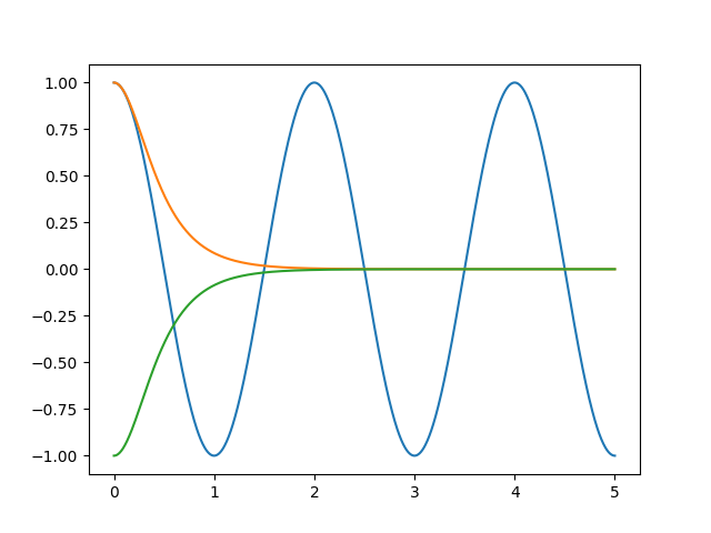
These two implicit equations don’t have analytical solutions. However, graphing \(\cos(\pi x)\) along with \(\pm 1 / \cosh(\pi x)\) shows us that the solutions quickly converge to the form \(n + 0.5\) for positive integer \(n\), and this convergence is very fast considering that \(\cosh\) exhibits approximately exponential growth.

It suffices to simply have the first few modes precomputed, and the rest approximated with integers + 0.5:

These approximations beyond these five precomputed values are accurate to well within 0.1 cents, so any deviations from the true solutions should be inaudible. Sonically, both beam models conform to odd harmonics but with the first few modes out of tune.

To account for the different effects of the position of excitation, you can use the mildly complicated formulas for the shape of the free-vibrating beams. This seems overkill to me though, and I think the simple sine wave-based formula of the clamped string should be good enough for a realistic sound.

This model is for a beam with uniform thickness, which is not the case with the arched keys of xylophones and vibraphones.

Rectangular and circular membranes

Membranes are found mainly in drum heads, and are modeled using a two-dimensional wave equation, making them a generalization of strings. With a two-dimensional resonator, we drop the mode number \(k\) and replace it two dimensions, \(m\) and \(n\), both positive integers.

A rectangular membrane clamped at the border has modal frequencies

where \(\alpha \geq 1\) is the aspect ratio of the rectangle, the ratio of the \(m\)-axis to the \(n\)-axis. Again, \(\propto\) indicates proportionality, and indicates that the right-hand side should be multiplied by the appropriate factor so that \(f_{1,1} = f_0\).

The most famous membrane equation is the circular membrane clamped at the edge, which has modal frequencies

where \(J_{(m - 1)n}\) is the \(n\)-th positive root of the Bessel function \(J_{m - 1}\). Bessel function zeros can be found with, for example, SciPy’s scipy.special.jn_zeros.

Amplitudes that take into account the strike point are also two-dimensional now. In the case of the rectangular membrane, the effect on membrane modes at the strike point \((x,y)\) is given by

The excitation position effects for the circular membrane are somewhat more complicated. For music purposes, I don’t see any issues with simply reusing the rectangular formula – the sonic effect is basically the same.

Rectangular plates and tubular bells

Just as membranes use the two-dimensional wave equation, rigid plates use a two-dimensional analog of Euler-Bernoulli beam theory.

The vibrations of rectangular plates have been well-studied, e.g. in [Leissa1973]. It’s well known that a clamped rectangular plate has resonant frequencies

Unfortunately, other boundary conditions like free plates result in partial differential equations with no known analytical solutions. However, if we simplify and treat each point of a plate as a superposition of two Euler-Bernoulli beams at right angles, we can work around this, sacrificing some accuracy. This was done in the tubular bell model of [Rabenstein2010], which arrives at

Modifications to Rabenstein’s model show how to derive the modal frequencies for a tube clamped at one end:

Or a plate that’s completely free:

Be warned: the above two are my own work, so I can’t necessarily guarantee that they’re correct!

Efficiency considerations

Modal synthesis is somewhat computationally expensive. Moore’s Law has increased the usefulness of modal synthesis over the years, but it’s still worth discussing how it can eat up CPU cycles and how we can mitigate that.

The models that we’ve discussed generate an infinite sequence of modes, but only a finite number of them will be in the audible range. Theoretically, we should be able to remove any modes if \(f_k \geq 20\,\text{kHz}\) (or the Nyquist limit if your sample rate is below 40 kHz), but this has two undesirable side effects:

• If you continuously modulate pitch, some modes will cross the 20 kHz threshold and will zap in and out of existence. This will create discontinuities in the output signal.

• Generally, lower pitches will require more modes, and you will get a different real-time CPU load depending on which note you play.

The first issue can be prevented by making a fake lowpass filter that smoothly crossfades modes to 0 as they approach 20 kHz. However, the second is a well-known issue in modal synthesis, and the best attack strategy depends on your design goals with regards to audio quality vs. CPU efficiency.

If deterministic CPU usage is a concern for you, it is probably wise to lose some bandwidth and simulate a fixed set of modes, say the lowest eight modes. It’s up to you to find out how much you can get away with before it starts degrading the output quality.

Standard strategies for reducing CPU cycles also apply. Modal synthesis doesn’t hurt particularly from downsampling. It’s also very ripe for vectorization and/or parallel computation on multiple threads.

Miscellany

Other physical models: If the resonances of an object can’t be easily solved with partial differential equations, you will have to use more powerful analytical tools like the Finite Element Method, which decomposes a body into a network of masses connected by springs, reducing mode identification to an eigenvalue problem. FEM is complicated in practice and I’m still trying to figure out how to implement it. MODALYS is one FEM tool designed for musicians, but it’s closed source, so I’m not really about that.

The Finite Element Method is not to be confused with the Finite Difference Method, where the model is discretized into a grid and simulated directly in the time domain.

909-style frequency sweep: Modal synthesis of drums benefits from a completely non-physical trick where the frequency is swept downward on the initial transient. This is an idea lifted from the Nord Drum, and reminds me of the kick drum in the Roland TR-909. My preferred envelope is \(f(t) = f_0 [1 + e(t)]\) where \(e(t)\) is an exponentially decaying signal.

Use as an audio effect: Modal synthesis isn’t just for impact percussion – a modal synthesis model can accept arbitrary audio input and take on the role of an effect, like a very metallic mini-reverb. In such cases, it’s usually a good idea to use significantly reduced decay times for better transparency, and/or introduce a dry-wet mix control.

Series and parallel: Used in Ableton Live’s Collision, multiple modal synthesis models can be combined. Layering is a given in sound design, and cascading multiple modal synthesizers can sound neat as well. You can do things such as simulating plucked strings attached to a wooden sound board.

Detuned copies: As seen in piano strings, Balinese gamelan, and EDM super saws, detuned copies of the same sound will thicken it and add evolution to the timbre. Modal synthesis in particular permits a computational shortcut as suggested in [Bank2010] – only the loudest modes require detuned copies to get the desired effect.

Feedback: This one’s easy – feed back the output of the summed modes into the excitation with a single-sample delay. Distortion or compression may be used in the feedback path.

Sum and difference tones: Modal synthesis is based entirely on treating resonances as linear filters, and doesn’t take into account nonlinear resonances that can happen in real objects. These are fiendishly hard to simulate, but there is a cool idea from [Bank2010] that allows us to simulate sum and difference tones that tend to arise from nonlinearities. For pairs of modes \(f_j,\,f_k\), create a new mode with frequency \(f_j \pm f_k\), loss factor \(R_j + R_k\), and amplitude \(A_j A_k\). (Be aware that multiplying the amplitudes of the modes now makes this model sensitive to scaling factors, since that is how nonlinearities work.) To avoid adding hundreds of new modes, it’s best to be selective and only do this for a small number of modes, such as the loudest three.

Other modifications: There are limitless variations possible here. There’s plenty of ad hoc modifications to experiment with, like detuning a single mode or removing it entirely. I’ll dump some open questions I thought of while working on this article. Can the beam, plate, and membrane models be augmented with additional controls to bring them more degrees of freedom? Are there ways to hybridize modal synthesis with other physical modeling techniques like digital waveguide synthesis? Is it possible to interpolate between different modal synthesis models, e.g. a drum that slowly morphs into a tube?

Conclusions

I have a confession to make: I haven’t actually tried realizing and listening every idea in this article. I wrote it only so that I can gather all this knowledge in one place. In practice, turning a mathematical formula into music requires skill in sound design. Creating interesting sounds with modal synthesis and employing them in a quality work of music is left as an exercise to the reader.

Thanks to Josh Mitchell for inspiring me to finish this article, which languished as a draft for a long time. I’d also like to thank the authors of the various citations for graciously allowing me to use their formulas without their permission.

References

Bilbao, Stefan. 2006. “Modal Synthesis.” https://ccrma.stanford.edu/~bilbao/booktop/node14.html
Rovan, Joseph Butch et al. “Instrumental Gestural Mapping Strategies as Expressivity Determinants in Computer Music Performance.”
Ren, Zhimin et al. 2012. “Example-Guided Physically Based Modal Synthesis.”
Chaigne, Antoine and Askenfelt, Anders. 1993. “Numerical simulations of piano strings. I. A physical model for a struck string using finite difference methods.”
Chaigne, Antoine and Askenfelt, Anders. 1993. “Numerical simulations of piano strings. II. Comparisons with measurements and systematic exploration of some hammer-string parameters.”
Gillet, Émilie. 2015. Source code of Mutable instruments’ “Elements.” https://github.com/pichenettes/eurorack/blob/2a468734bdd53bea0f25165bf34d92a4c571db13/elements/dsp/resonator.cc#L64
Bank, Balázs et al. 2010. “A Modal-Based Real-Time Piano Synthesizer.” IEEE Trans. on Audio, Speech, and Language Processing.
Stoelinga, Christophe N. J. and Lutfi, Robert A. “Modeling manner of contact in the synthesis of impact sounds for perceptual research.” Journal of the Acoustical Society of America.
Chaigne, Antoine and Doutaut, Vincent. 1998. “Numerical simulations of xylophones. I. Time-domain modeling of the vibrating bars.” https://asa.scitation.org/doi/abs/10.1121/1.418117
Leissa, A. W. 1973. “The free vibration of rectangular plates.” Journal of Sound and Vibration. https://www.sciencedirect.com/science/article/pii/S0022460X73803712
Rabenstein, Rudolf et al. 2010. “Tubular Bells: A Physical and Algorithmic Model.” IEEE Transactions on Audio, Speech, and Language Processing.