Audio Effects with Wavesets and K-Means Clustering
(original)
(processed)
I would like to congratulate wavesets (not wavelets) for entering their 30th year of being largely ignored outside of a very small circle of computer music nerds. Introduced by Trevor Wishart in [Wishart1994] and popularized by Microsound [Roads2002] and the Composers Desktop Project, a waveset is defined as a segment of an audio signal between two consecutive upward zero crossings. For simple oscillators like sine and saw waves, wavesets divide the signal into pitch periods, but for general periodic signals there may be any number of wavesets per period. For signals containing noise or multiple pitches at once, waveset segmentation is completely unpredictable.
Many simple audio effects fall out of this idea. You can reverse individual wavesets, omit every other waveset, repeat each waveset, sort them, whatever.
I like waveset-based effects best on input signals that are monophonic (having only one pitch) and low in noise. Synthetic signals can make for particularly interesting results. Much as the phase vocoder tends to sound blurry and phasey, waveset transformations also have their own “house style” in the form of highly digital glitches and crackles. These glitches are particularly pronounced when a waveset-based algorithm is fed non-monophonic signals or signals containing strong high-frequency noise. Wavesets are extremely sensitive to any kind of prefiltering applied to the input signal; it’s a good idea to highpass filter the signal to block dc, and it’s fun to add pre-filters as a musical parameter.
Today, we’re putting a possibly new spin on wavesets by combining them with basic statistical learning. The idea is to perform k-means clustering on waveset features. The steps of the algorithm are as follows:
Segmentation: Divide a single-channel audio signal into \(N\) wavesets.
Analysis: Compute the feature vector \(\mathbf{x}_i\) for the \(i\)-th waveset. I use just two features: length \(\ell_i\), or number of samples between the zero crossings, and RMS \(r_i\) of the waveset’s samples. All the lengths are compiled into a single size-\(N\) vector \(\mathbf{\ell}\) and the RMSs into \(\mathbf{r}\).
Normalization: Scale \(\mathbf{\ell}\) and \(\mathbf{r}\) so that they each have variance 1.
Weighting: Scale \(\mathbf{\ell}\) by a weighting parameter \(w\), which controls how much the clustering stage emphasizes differences in length vs. differences in amplitude. We’ll talk more about this later, but \(w = 5\) seems to work as a start.
Clustering: Run k-means clustering on the feature vectors \(\mathbf{x}\), producing \(k\) clusters.
For each cluster, pick one representative waveset, the one closest to the centroid of the cluster.
Quantization: In the original audio signal, replace each waveset with the representative waveset from its cluster.
Implementation is very lightweight, clocking in at about 30 lines of Python with scikit-learn. There are only two parameters here other than the input audio: \(w\) and \(k\). [1] The length of the input audio signal is important too, so for musical reasons let’s not think in terms of \(k\) but rather “clusters per second” \(c\), which is \(k\) divided by the signal length in seconds. As we will see, with only two-dimensional control we can produce a tremendous variety of sounds.
Exploration
I started with an a cappella cover of “Stay With Me” by a singer named Aiva, which I use often for testing monophonic algorithms. This segment is 17 seconds long, 44.1 kHz — as I mentioned, the length of the audio file is important.
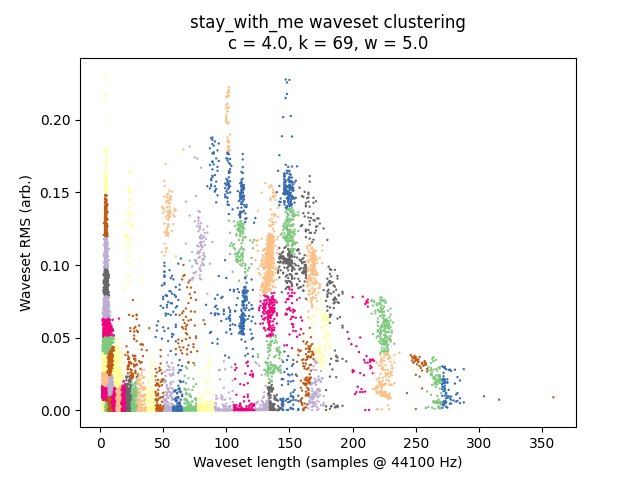
This file splits into about 26,000 wavesets. Running the algorithm with \(w = 5.0\) and \(c = 4.0\):
The pitch content is retained, but the voice is now speckled with all kinds of glitchy mutations. (As an aside, sklearn.cluster.KMeans crunches it in a fraction of a second, and I have no concerns with efficiency.)
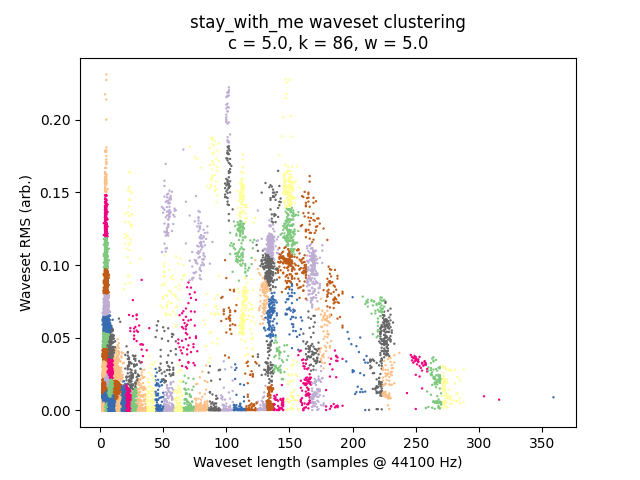
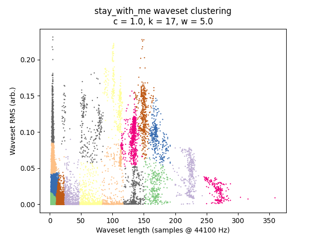
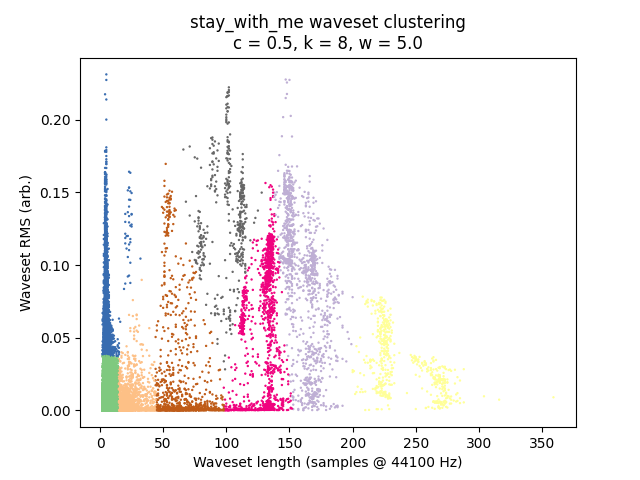
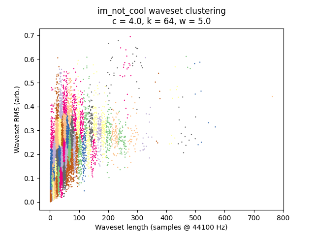
It is always instructive to look at plots if we can, and in this case it is quite easy given that we have only two-dimensional data to plot. I’ve placed waveset duration on the X-axis and waveset RMS on the Y-axis, and assigned each cluster to a random color. (Sorry, some different clusters might have similar-looking colors.)
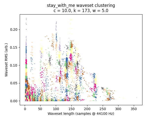
\(c\) is the most important parameter here — let’s reduce it, which changes the severity of the glitches.
\(c = 10.0\):
\(c = 5.0\):
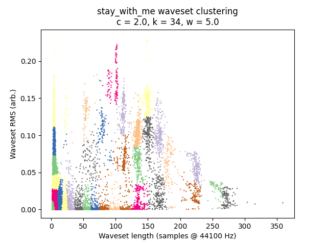
\(c = 2.0\):
\(c = 1.0\):
\(c = 0.5\):
We also have \(w\) to tune, which affects the “warbliness” of pitch. Higher \(w\) values result in clusters forming more vertically, while lower values result in more horizontal stripes. For the sake of space, I will not demonstrate this tuning here; I don’t find it a particularly musical parameter to tune and prefer to leave it at 5.
Trying on different audio files
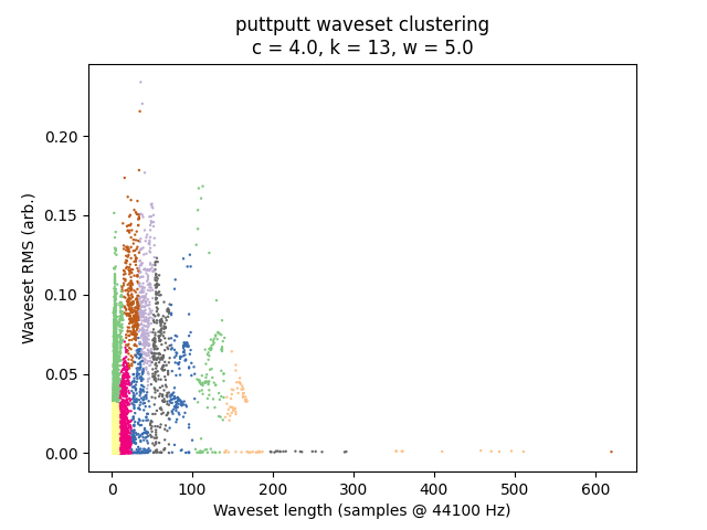
This algorithm is highly signal-dependent, and worth trying on a wide variety of audio files. Here are just a few. The morphology of the 2D plot is particularly interesting.
Speech
Singing tends to hover around quantized pitches, but speech does not, and the clustering algorithm is aware of this. The effect on pitch is particularly interesting here, and very squelchy. (This is perhaps not a fair comparison because this file is considerably shorter than the sung example.)
(original)
(processed)
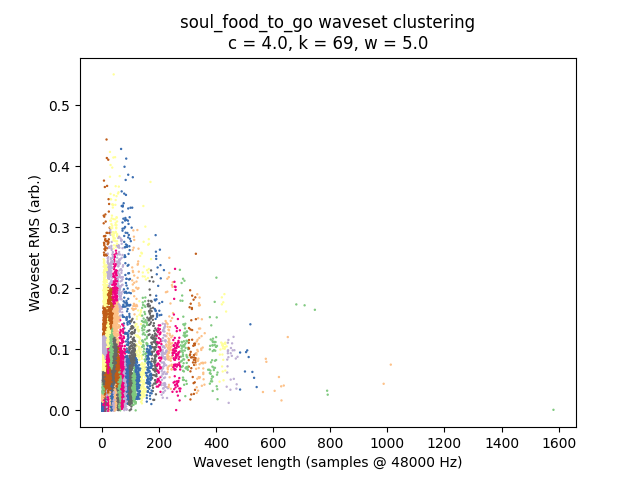
Percussion
Manhattan Transfer’s “Soul Food to Go” sounds like a Clipping beat.
(original)
(processed)
Full mix
Scott Krippayne’s “I’m Not Cool” turns into digital soup.
(original)
(processed)
Discussion
No question this could be done in real time, by performing k-means on a sliding window of the last N seconds of wavesets. There is considerable literature on “streaming k-means” algorithms [Ailon2009], but for our application the accuracy of clustering is not too important and simply re-running an iteration step of the standard k-means algorithm might work fine. Now imagine filtering it with EQ to screw up the zero crossings, and routing it back into itself with a delay.
I messed a bit with expanding the contextual information of the feature vectors, adding the features of nearby wavesets (with reduced weights so they have less impact on the clustering). However, I was pleased enough with the context-free wavesets that I decided not to push this. I also feel there are other approaches to context that are perhaps more immediately musical. You could for example train a Markov chain on the sequenced wavesets.
This use of clustering is known as vector quantization (VQ), where a vector is replaced with the closest one in a “codebook” of vectors. A very important application of VQ is compression, so it appears commonly in lossy codecs, including audio codecs where it is often used to quantize speech parameters (see Code-Excited Linear Prediction).
Another precedent for what we’re doing here is concatenative synthesis [2], whose standard pipeline involves segmenting audio, analyzing the segments to produce feature vectors, and performing any manner of statistical operations on said feature vectors. Maybe I didn’t look hard enough, but I was unable to find anyone combining wavesets with concatenative synthesis. I did find that a lot of concatenative synthesizers pile on all sorts of fancy machine listening features. There’s nothing wrong with doing that, but the success of the method presented here demonstrates that a “dumb” algorithm — in this case an elementary segmentation method and just two features — is fully capable of sounding distinctive and musical.
Footnotes
References
Wishart, Trevor. 1994. Audible Design.
Roads, Curtis. 2002. Microsound.
Ailon, Nir et al. 2009. “Streaming k-means approximation.” https://proceedings.neurips.cc/paper/2009/hash/4f16c818875d9fcb6867c7bdc89be7eb-Abstract.html