Ring modulation of real signals

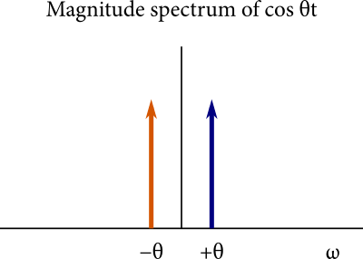
A real audio signal \(f(t)\) has a Fourier transform satisfying \(F(-\omega) = F(\omega)^*\), i.e. all negative frequency content is the complex conjugate of the positive frequency content. An individual sine wave \(\cos \theta t\) produces Dirac delta-shaped spikes in the frequency spectrum at \(\theta\) and at \(-\theta\). To illustrate, here is a depiction of the absolute value of such a spectrum vs. angular frequency:

The Fourier transform has a convolution theorem, where convolving two signals in the time domain is identical to multiplying them in the frequency domain. Critical to understanding the frequency-domain behavior of ring modulation is the counterpart:

Multiplying two signals in the time domain is identical to convolving them in the frequency domain.

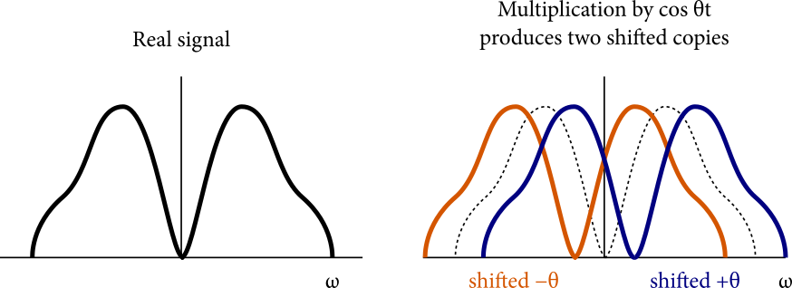
A ring modulator mutliplies a signal \(f(t)\) by a sinusoid \(\cos \theta t\). [1] By performing convolution of these two signals in the frequency domain, we get two sidebands: \(f(t)\) frequency shifted up by \(\theta\), and \(f(t)\) frequency shifted down by \(\theta\). This is because convolution with a shifted Dirac delta function is a horizontal shift.

Here’s what it looks like visually. The left diagram is the magnitude spectrum of some arbitrary real signal, and the right shows the magnitude spectra of the two shifted copies:

(Sorry about the goofy-looking diagrams in this post. I wanted to make them more professional, but that took too much work.)

The ring modulator is already almost a frequency shifter, but it produces two shifted copies. What if there was a way for a ring modulator to produce only one sideband? Hmmm…

Frequency shifting of analytic signals

Most audio signal processing concerns real signals, so it’s easy to forget that they are a subset of the larger domain of complex signals. A complex signal \(A + jB\) can be represented in analog or digital environments using two real signals, one for the real part \(A\) and the other for the imaginary part \(B\). In the frequency domain, complex signals are not beholden to the constraint that real signals have on negative frequencies. Their positive spectrum can be completely independent of the negative spectrum.

In frequency shifting, we are interested in a subset of complex signals called the analytic signals. A complex signal \(f\) is analytic if \(F(\omega) = 0\) for all \(\omega < 0\). [Smith2007] That is, the Fourier transform of \(f\) has no negative frequency content.

Why is this useful for frequency shifting? While real signals decompose into real sinusoids of the form \(A \cos(\omega t + \phi)\), the building block of an analytic signal is the complex sinusoid, which has the general form \(A e^{j (\omega t + \phi)} = A \cos(\omega t + \phi) + A j \sin(\omega t + \phi)\), where \(A \geq 0\), \(\omega \geq 0\), and \(0 \leq \phi < 2\pi\). Instead of the dual spikes of the real sinusoid, a complex sinusoid’s spectrum is a single spike at a positive frequency.

Since multiplication in the time domain is convolution in the frequency domain, multiplying by a complex sinusoid \(\cos \omega t + j \sin \omega t\) convolves with a single Dirac delta function at \(\omega\). The lack of negative frequency content means that only the upper sideband is generated. That’s a frequency shift by \(\omega\).

This even works if the complex sinusoid has negative frequency. Although the shifting process crashes into DC and generally produces a non-analytic signal, this isn’t an issue.

A ring modulator multiples a real signal by a real sinusoid, while a frequency shifter (or at least our specific design of it) multiplies an analytic signal by a complex sinusoid.

There is one fundamental property of analytic signals that we need to know before we proceed. The imaginary and real parts of an analytic signal have a special relationship: the imaginary part is the Hilbert transform of the real part of the signal. The Hilbert transform of a signal is a “constant -90-degree phase shift,” or more accurately, a -90-degree phase shift of all positive frequency content and a +90-degree phase shift of all negative frequency content (the latter is to ensure the signal stays real). [2] The Hilbert transform property of analytic signals can be easily proven from the definition of the Fourier transform.

Borrowing terms from telecommunications, analytic signals are often known as “quadrature signals” or “\(I/Q\) signals.” The real part of the signal is denoted \(I\) (for “in-phase”) and the imaginary part \(Q\) (“quadrature”).

Converting between analytic and real signals

So, nice. Analytic signals allow for easy implementation of a frequency shifter. So how do we convert from real to analytic signals and vice versa?

Converting from complex signals back to real signals is trivial. We just drop the imaginary part:

To convert from real to analytic, we can try using a Hilbert transform to construct the imaginary part:

Unfortunately, the Hilbert transform is noncausal, with an impulse response that tails infinitely in both directions. In digital settings, FIR filters are a common approach for approximating the Hilbert transform (with some latency that has to be compensated with a delay line in the \(I\) signal). The literature on this is extensive thanks to Software-Defined Radio applications: just search for “Hilbert FIR.”

In the analog domain, an IIR filter method exists for converting a real signal to an analytic one: a “90-degree phase-difference network.” Rather than directly implementing the Hilbert transform as a filter, a phase-difference network takes an input signal X and puts it through two parallel allpass filters, producing two signals A and B such that B is roughly the Hilbert transform of A. “Roughly” means that the phase shift of B relative to A is close to -90 degrees over a useful bandwidth, say 20 Hz to 20 kHz.

The allpass filters are formed from a cascade of one-pole one-zero allpass filters, each having the following transfer function:

where \(p\) is real and negative, representing the location of the pole. How do we select the locations of the poles? The mathematics are beyond me, but there is a published algorithm for optimal design of such filters described in [Weaver1953] and elaborated on in a well-known document from ElectroNotes [Hutchins]. The algorithm receives minimum and maximum frequencies to define the operating bandwidth, and you can either specify the number of allpasses (“design a network with \(n\) poles”) or the error in the phase difference (“design a network with less than \(E\) degrees of deviation from 90 degrees”). I wrote up some Python/NumPy code for this, available at the end of the post.

If we specify the operating range as 20 Hz to 20 kHz, a phase difference network with 12 poles, six in each path, can achieve less than 2 degrees of deviation from 90 degrees in the audio frequency range. Here are the locations of the poles that I get (units in radians/second):

Poles, path A:
    -45.363318968136156
    -344.47613274064236
    -1402.0629595305616
    -5624.48591607002
    -22572.489209831336
    -100338.8419291972
Poles, path B:
    -157.380399635128
    -699.584653466801
    -2807.6107358762515
    -11262.951449077736
    -45841.68695841799
    -348108.72310368466

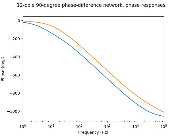
I skipped an important detail. Maybe A and B are almost 90 degrees apart, but how do they relate to the input signal? The relationship isn’t straightforward, so a graph will help. Both branches of the network are allpass filters, meaning that their gain is unity at all frequencies, so only their phase responses are worth looking at. Let’s plot the phase response of Allpass A and Allpass B:

Here’s the phase difference between Allpass A and Allpass B to show how close we are to -90 degrees:

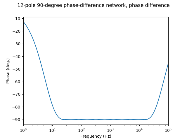
Good enough for our needs. (Open question for readers: how low does this error need to be for it to be inaudible in the resulting effect?)

The Complete Frequency Shifter

We’ve now defined conversion processes between analytic and real signals, and we have all the tools needed to complete our frequency shifter:

• Convert rom a real signal to an analytic signal \(I + jQ\).

• Multiply by a complex sinusoid.

• Convert the complex signal back to a real signal.

Note that the modulation step, the multiplication must be complex multiplication. If the input signal is \(I + jQ\), complex multiplication expands as follows:

But since we’re immediately converting back to a real signal, the imaginary term doesn’t matter, and we just need to compute \(I \cos \omega t - Q \sin \omega t\). That completes the block diagram of our analog frequency shifter:

This is only a block diagram. Fleshing this out into actual analog schematics is an entirely different story, and I won’t claim any expertise in that. Again, just check out [Haible1996] for yourself.

Digitization

Analog one-pole filters are simple to digitize using the bilinear transform.

where \(k = \frac{p + 2f_s}{p - 2f_s}\), where \(f_s\) is the sample rate and \(p\) is the location of the analog pole. Even without pre-warping, this achieves excellent agreement to the analog phase response, and it’s not worth fretting over inaccuracies in my opinion.

Antialiasing is a valid concern when working with digital frequency shifters. With positive frequency shifts, frequency content may be shifted above Nyquist. This can be countered by pre-application of a lowpass filter at \(f_s / 2 - f\) if frequency shifting upward by frequency \(f\).

Variations

We have a nice-sounding frequency shifter based on an established algorithm in signal processing. What twists can we add to give it some unique character?

In an analog design, the one-pole allpass filter is typically an active design containing an op-amp. Op-amps can be a source of nonlinearity, so this suggests a “dirty” frequency shifter with waveshaping after each allpass stage. [3] The sine wave modulator signal can also be made non-ideal with harmonic distortion or temperature drift.

I don’t think it’s worthwhile to do exact modeling of every nonlinearity and imperfection in an analog frequency shifter. All I am suggesting here is that effect design doesn’t need to stop at an idealized mathematical model, and that there is a potentially interesting space to explore in deliberately imperfect frequency shifters, especially using imperfections directly inspired by analog circuits.

Conclusion

Python/NumPy code for designing the phase difference networks and making the plots is available on GitHub. Admittedly I haven’t done a lot of work to verify its correctness, so please let me know if you discover errors.

Edit 2020-03-06: I mistakenly claimed that the phase responses of the allpass filters are nearly linear, completely forgetting that the X-axis of the plot is logarithmic. Oops. I’ll put up a graph of the group delay if I have time.

References

Actually

References

Boschen, Dan. 2016. Answer on DSP StackExchange. https://dsp.stackexchange.com/a/31360
Boschen, Dan. 2020. Answer on DSP StackExchange. https://dsp.stackexchange.com/a/63812
Weaver, Donald K. 1953. “Design of an RC Wide-Band 90-Degree Phase-Difference Network.”
Hutchins, Bernie. “The Design of Wideband Analog 90° Phase Differencing Networks Without A Large Spread of Capacitor Values.” http://electronotes.netfirms.com/EN168-90degreePDN.PDF
Haible, Jürgen. 1996. “JH FS-1 Frequency Shifter.” http://www.jhaible.info/tonline_stuff/hj_fs.html
Smith, Julius O. 2007. “Analytic Signals and Hilbert Transform Filters.” https://ccrma.stanford.edu/~jos/r320/Analytic_Signals_Hilbert_Transform.html