Correlated Granular Synthesis
Decades after Curtis Roads’ Microsound, granular synthesis is making appearances here and there in the commercial plugin market. While it’s nice to see a wider audience for left-field sound design, I have my quibbles with some of the products out there. From what I’ve heard, so many of these products’ demos are covered in reverb in obvious compensation for something, showing that the plugins seem most suited for background textures and transitional moments. In place of sound, the developers seem to prioritize graphics — does watching 3D particles fly around in a physics simulation inspire the process of music production, or distract from it?
Finally, and most importantly, so many granular “synths” are in fact samplers based on buffer playback. The resulting sound is highly dependent on the sampled source, almost more so than the granular transformations. Sample-based granular (including sampling live input such as in Ableton Live’s Grain Delay) is fun and I’ve done it, but in many ways it’s become the default approach to granular. This leaves you and me, the sound design obsessives, with an opportunity to explore an underutilized alternative to sampled grains: synthesized grains.
This post introduces a possibly novel approach to granular synthesis that I call Correlated Granular Synthesis. The intent is specifically to design an approach to granular that can produce musical results with synthesized grains. Sample-based granular can also serve as a backend, but the idea is to work with the inherent “unflattering” quality of pure synthesis instead of piggybacking off the timbres baked into the average sample.
Correlated Granular Synthesis is well suited for randomization in algorithmic music context. Here’s a random sequence of grain clouds generated with this method:
Grainlet synthesis
In Microsound, Roads describes a granular synthesis technique he calls grainlet synthesis. (Dude sure likes neologisms.) Inspired by how wavelets couple frequency with duration, grainlet synthesis refers to any kind of granular synthesis where “parameter linkage” is present. He illustrates with a directed graph of parameters, with arrows showing the dependencies between parameters:
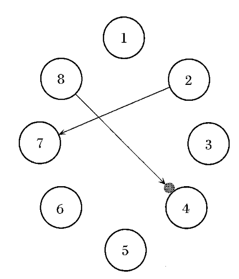
The description is light on details, but as far as I can fathom, the parameters are mostly randomized while parameters with dependencies are compute deterministically from other parameters. In the above diagram, we have parameter 2 controlling parameter 7, so after randomizing parameter 2 for a given grain, parameter 7’s value is found by computing an increasing function of parameter 2’s value. The arrow from 8 to 4 has a gray circle on it indicating inverse linkage – as parameter 8 increases, parameter 4 decreases.
Roads’ grainlet diagram popped into my head recently, and I realized that the trichotomy of linkage vs. inverse linkage vs. no linkage is really a special case of the general concept of correlation in statistics. Thus, Correlated Granular Synthesis was born: granular synthesis where grain parameters are generated by sampling a multivariate probability distribution.
Overall, where many extant granular synthesis methods are opinionated about DSP algorithms, Correlated Granular Synthesis is opinionated about how parameters are set. Thus it really serves as a frontend to granular synthesis methods, allowing us to imagine Correlated Glisson Synthesis, Correlated Trainlet Synthesis, Correlated Pulsar Synthesis, Correlated Vosim Granular Synthesis, etc.
Absolute time as a grain parameter
“Density” (e.g. average grains per second) is a critical parameter for any granular synthesizer. While experimenting with Correlated Granular Synthesis, I realized there’s an alternative characterization where instead of density, we directly think of the absolute timestamp of the parameter as a parameter just like pitch, amplitude, etc.
A traditional granular synthesis approach is to consider all parameters modulatable over time, and these modulations are left up to the composer or performer. In Correlated Granular Synthesis, time is just another grain parameter, and if a non-time parameter “modulates” it’s really a special case of statistical correlation. An important implication is that Correlated Granular Synthesis is a more or less offline sequencer where all grains have to be planned out in advance, although the synthesis itself can be in real time.
Selecting probability distributions
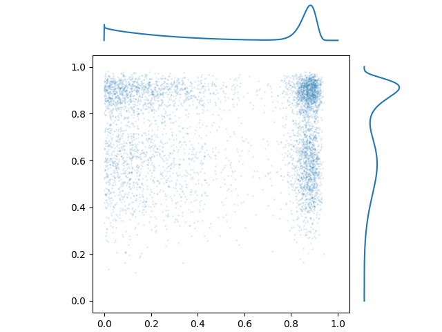
Before we start correlating anything, let’s first pick out the marginal probability distributions. In a multivariate probability distribution, a marginal PDF is what you get when you ignore all variables but one. Here’s a 2D probability distribution with the marginal PDFs displayed:
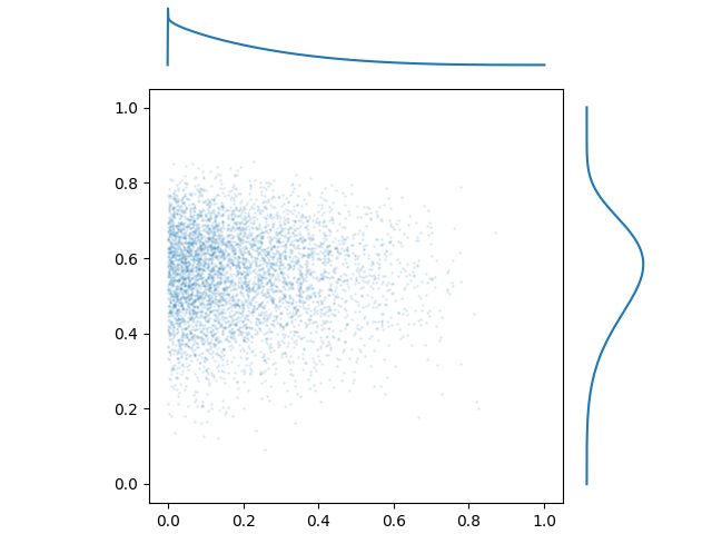
In this case, the sampling process is independent for each variable. The Pearson and Spearman rank correlations are both very close to 0, and there isn’t any interaction between these features. We’ll address that soon, but first, let’s talk about the marginal distributions themselves.
To simulate a univariate probability distribution, a simple and general method is to use inverse transform sampling. If \(X(x)\) is the probability distribution function, then we define the cumulative distribution function \(F(x) = \int_{-\infty}^x X(t) dt\). Most importantly, the inverse CDF \(F^{-1}(x)\) (a.k.a quantile function) takes a uniformly distributed random variable in the range \([0, 1]\) and transforms it to a variable with PDF \(X\).
Not all distributions have a guaranteed closed-form inverse CDF. In the worst case, we can numerically integrate \(X\) and construct a table of values to approximate the inverse CDF. We can even let the user draw their own PDFs, although that strikes me as excessive. Personally, I value simplicity of implementation, so my preferred approach is to select probability distributions that already have a nice closed-form inverse CDF and supply some parameters that let us mess with the shape.
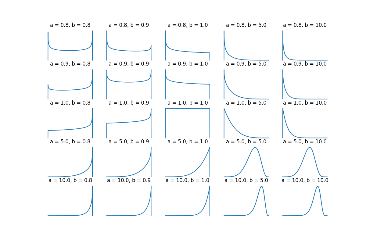
I like bounded distributions because it’s easier to control wacky values. Out of established bounded distributions with at least one shape parameter, the Kumaraswamy distribution
has two shape parameters \(a,b > 0\) and a closed form inverse CDF:
As for what the shape parameters actually do, it’s a bit hard to describe, but here’s a plot of some PDFs:
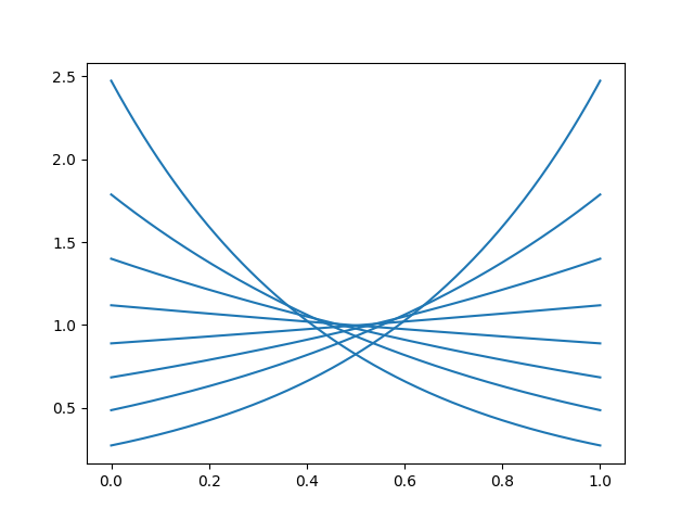
Another bounded distribution with a nice inverse CDF is the continuous Bernoulli distribution:
with inverse CDF
where \(X_C^{-1} = -\frac{\log [-x / ((\lambda - 1) N(\lambda)) ]}{\log (1 - \lambda) - \log \lambda}\) and \(N(\lambda) = \frac{2\tanh^{-1}(1 - 2\lambda)}{1 - 2 \lambda}\), if WolframAlpha has not failed me. \(0 < \lambda < 1\) is the shape parameter. The shape parameter is easier to describe here, it just tilts the PDF:
Both these distributions are defined for \(x \in (0, 1)\) and must be scaled to the appropriate range.
It’s tempting to use a single highly general distribution with many shape parameters, but I’d recommend having multiple types of distributions that do one thing well with a small number of parameters. This gives us the benefits of the switching principle.
Introducing correlation with linear transformations
The simplest way to add correlation is to use a linear transformation: sample an independent random variable \(\mathbf{x}\), then put it through a matrix \(\mathbf{x}' = \mathbf{A}\mathbf{x}\).
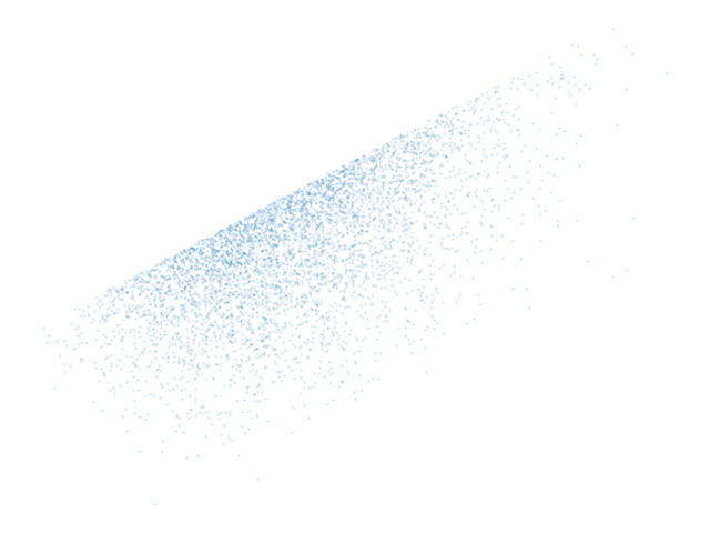
That’s it, we have correlation. If you imagine the x-axis as time and the y-axis as frequency, this is an upward sweep. I’ve gotten good results just randomizing the matrix \(\mathbf{A}\) with a uniform distribution, and using tanh to bias it a bit away from zero.
(In the special case where all variables have independent standard normal distributions, the correlation matrix is given as \(\mathbf{K} = \mathbf{A}\mathbf{A}^\top\), and you can actually recover \(\mathbf{A}\) from \(\mathbf{K}\) using the Cholesky decomposition. While the math of correlation in multivariate distributions is quite deep, in practice we don’t need any of that to make interesting granular synths.)
If you don’t introduce any correlation between variables but do select interesting probability distributions, the result doesn’t necessarily sound bad either:
Here’s the audio from the top of the post again, for comparison:
Both samples use the same DSP (windowed hard-synced sine waves), the only difference is the selection of multivariate distributions. Chalk it up to confirmation bias, but to me the second sample is livelier and has a stronger sense of motion and gesture.
Mixture distributions
A fun thing to do is to use marginal PDFs that have multiple local minima and maxima. Here’s an independent 2D distribution:
There aren’t really any established parametric distributions that are capable of even these simple shapes, but it is possible to combine any number of distributions using a mixture. Mixture distributions are defined by a finite number of component distributions \(D_1, D_2, \ldots, D_n\) and a number of mixing weights \(w_1, w_2, \ldots, w_n > 0\) that all sum to one. To draw a single sample from a mixture distribution, pick a number \(1 \leq k \leq n\) with probability \(w_k\), and sample from distribution \(D_k\).
Kernel smoothing
Mixture models combine multiple probability distributions by randomly choosing between them for each sample. An alternative approach is to instead add together two or more independent random variables, possibly with weights. A well-known result of probability theory is that the addition of random variables results in convolution of their PDFs. If one of the PDFs is normal or roughly normal-shaped, it acts as a lowpass filter and diffuses the PDF. This is known as kernel smoothing.
Nonlinear warping
It’s also possible to warp the data nonlinearly with whatever crazy functions you want. Here’s what I got throwing some random functions together including a Möbius transformation and a Cartesian-to-polar conversion for some reason:
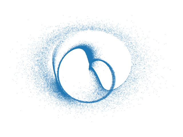
As fun as this looks, this kind of visual is of limited use for higher-dimensional PDFs, and the sound is more important anyway. Given that the number of possible formulas is basically unlimited, algorithmic methods are advisable for navigating this space.
Conclusion
This is another synthesis post where I’ve put in the minimal work to get to sounds that I find interesting, but made very little effort to design an intuitive interface. (That’s generally how things go for this blog: research first, development eventually.) As I said, this method is well suited to randomization — the sort of thing where you keep changing the seed until you get a result you like. How to produce an interface is a tough question, because there are so many parameters and it’s hard to predict what settings are musical.
During the creation of this post, I researched standard methods for simulating multivariate normal distributions and landed on something called a Gaussian copula. An earlier and much longer version of this post involved a detailed explainer on how Gaussian copulae work, but when I actually listened to their effects, it became clear that there wasn’t any particular reason to bring them into the picture. (Interestingly, Gaussian copulae, or misuse of them, are said to have played a role in the 2008 financial crisis.) Ad hoc approaches to designing multivarite PDFs not only require less effort, but sound better. Lesson learned: before spending multiple days writing about something, it’s best to implement and listen to it first.